Author: Megan Strachan

This paper applies the use of convolutional neural networks (CNNs) in Fourier ptychographic microscopy to video capture.

Deep learning approaches to FPM, which computationally enhances the resolution of an image while maintaining a large field of view, have developed to replace the iterative model-based design. The neural net is preferable because once it has defined the relationship between low resolution inputs and the corresponding high resolution FPM output, it can transform input into output directly. The model based approach, in contrast, must iteratively improve its approximation of the high resolution object — a much slower process.

Nguyen et al. train a conditional generative adversarial network (cGAN) to determine the relationship between inputs and FPM output. One sub-network generates predicted FPM output, and the other sub-network attempts to decide whether the output is the ground-truth image or a prediction.

To apply this technique to video reconstruction, Nguyen et al. first assume that the samples on which they train display a sufficient quantity of cells that, within a single video frame, all cell states are represented somewhere. They then choose to train their CNN only the first frame of each video.

When the CNN is applied, frame-by-frame, to the remainder of the video, it is able to reconstruct each cell as it moves through many different states. This is because the original training frame exposed the CNN to all the possible conditions of a cell.

They treat each video frame as temporally independent of preceding frames. Because they know in what way cells of each state are meant to be reconstructed (by training on the many states present in frame 0), they simply reconstruct each state where it appears.

Using transfer learning, they are able to quickly train their model on new types of cells.

This technique for FPM video capture is a faster and more useful strategy than performing iterative FPM on each frame of a video. It has limitations, however. For a sample of cells too sparse or too large to all possible states within a single image, the strategy of only training on the first image of the video is ineffective. For fast moving samples, it will not be possible to collect a full low resolution input dataset before the cells change position.

Classification

• A linear regression model generates the decimal probability of an event occurring. To map this probability to a binary category (the event will or will not occur), you must define a classification threshold

o   The classification threshold decides which probabilities are associated with one and which are associated with zero

• You don’t always need a classification threshold. If you want to predict the probability of rain, you can just return the prediction as the decimal likelihood of rain.
• If, however, you want to predict if someone will or will not need a raincoat, you’ll need to decide which rain likelihoods should correspond to “raincoat” and which correspond to “no raincoat”

o   Threshold tuning considers the consequences of different types of incorrect predictions

• True positive means the model makes a correct positive prediction
• True negative means the model made a correct negative prediction
• False positive means the model incorrectly predicted the outcome as positive
• False negative means the model incorrectly predicted the outcome as negative
• False positives and false negatives have different consequences
• It is better to bring a raincoat and not need it (false positive) than to get caught out in the rain without one (false negative)

Prediction Bias

• Prediction bias occurs when the average of all predictions made by a model is not equal (or approximately equal) to the average of the dataset

o   Ex: if 10% of all dogs in a shelter are labs, the model should predict that a dog is a lab ~10% of the time

o   If avg. prediction – avg. observation is not zero, the model is biased

• Calibration layers to correct bias are a bad idea

o   It is possible to correct bias with brute force (for an 8% bias, add a layer that brings down the prediction mean by 8%)

o   This isn’t good because prediction biases signal that something is going wrong inside your model – it’s important to identify the actual problem instead of painting over it

• Overly regularizing data, using biased training data, or training on very noisy data are common causes of prediction bias

Regularization

• When sparse features are crossed, the model size becomes needlessly large, slowing down operations and using up memory

o   Extraneous weights should be made equal to 0 to save space and improve speed

• L1 regularization penalizes the absolute value of the sum of all weights in the model

o   It causes some weights to be zeroed out completely, unlike L2 regularization which works to keep weights near zero but does not eliminate them entirely

 

From Google’s machine learning crash course

Many deep learning frameworks are available to accomplish the same task in slightly different ways. Below, we summarize some key points from the most popular frameworks.

Tensorflow is the most widely used deep learning framework. It is developed by Google. Tensorflow is highly documented and Google offers extensive tensorflow-based machine learning training lessons and exercises for beginners. Tensorflow has its own visualization tool, tensorboard.

Tensorflow is not as fast as some other frameworks and has a reputation for being very complicated for beginners.

Pytorch is the second-most popular framework, after tensorflow. Pytorch is the python based variety of a deep learning framework called Torch and is developed by Facebook. Pytorch is known for being fast and efficient and is popular with researchers. It is more intuitive for new users than tensorflow.

Pytorch documentation is limited, and it does not have any inbuilt visualization tools (e.g. tensorboard)

Keras is a  simple, high level library developed primarily by a Google engineer named François Chollet. It works on top of frameworks like tensorflow and makes developing simple neural networks much easier for beginners.

Because Keras is meant to abstract the details of more in-depth libraries, it offers less control in building models.

MXNet is an effective framework, highly scalable framework used by AWS and other industry giants.

Documentation is more limited than other languages, which makes it a poorer choice for beginners.

Other options include Caffe (or Caffe2), Microsoft Cognitive Toolkit, and Deeplearning4j. All of these options are high performing but less well documented.

Most of the canonical choices of machine learning framework have comparable performance. Differences in speed and efficiency do not seem marked enough between the frameworks to strongly prefer one or another on that basis.

Instead, because our lab is not experienced in machine learning, we think it would be best to choose a well documented language with an active support community. We have explored Google’s tensorflow-based machine learning crash course for an introduction to the main concepts of machine learning and an overview of tensorflow use. Using keras with tensorflow may be a good choice for our collective skill level, with the option to transition to regular tensorflow for finer control as we become more experienced.

Links to useful data collection and processing documentation

Image Collection Procedure
Image Preprocessing and Reconstruction Procedure
Shift-Add Optimized Element Data Processing Procedure
Virtual Environment Setup

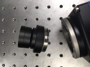
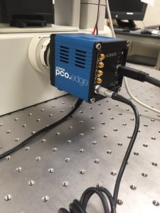
The Arduino and pco camera were unplugged from the power strip and the usb ports of the laptop. The picture below shows the camera attached to the microscope. The black and sliver cables were both removed.

Next, the camera was removed from the C mount of the microscope. The C mount adapter was removed from the camera so that a protective cover could be placed over the lens.

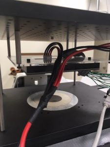
The LED matrix is affixed to an acrylic baseplate that is suspended above the microscope stage. The red and black wires are connected to the power supply, and were unplugged first. The acrylic baseplate was unscrewed from the top of the microscope.

A wiring guide for the 32×32 LED matrix may be found here . The jumper wires were disconnected from the LED array so that the Arduino could be packaged separately.

 

To reassemble the microscope, the LED array must be rewired and reaffixed to the top of the microscope. The array should be reconnected to the power supply and the Arduino should be reconnected to the USB port of the controlling computer.

The C mount must be reattached to the camera, which should also be reconnected to power and the laptop.

 

 

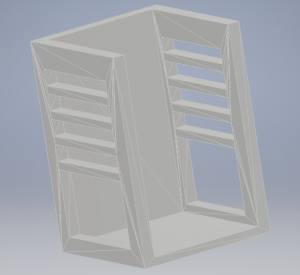
Our microscope assembly includes an LED array, foldscope lenses, and a cellphone. The first design for our microscope stand used a LEGO base to hold the LED array in place beneath the foldscope and cellphone arrangement, which were supported by a piece of cardboard. The second design, shown below, was made in Autodesk and 3D printed in the college makerspace.

The base of the stand is scaled to snugly hold the LED array in place. The four narrow supports along the sides of the stand are intended to hold the phone, foldscope, and slide assembly in place at four different heights, allowing for very crude z-distance adjustment.

Because the 3D design is uncomplicated, it was decided that future prototypes should be made of laser cut acrylic pieces and fitted together. The 3D printing job was too large to print on a practical timetable, and during early prototyping stages rapid iteration is desirable. The laser cuts take only a few minutes at a time, while the 3D print job took more than 24 hours.

This simple stand design was useful for developing skills in Autodesk and 3D printing, and for holding the microscope setup steady while attempting to take calibration images. However, it does not allow any fineness in z-distance adjustment and no movement at all in the x and y directions. Future designs will include 3 stepper motors arranged so that minute changes can be made in all three directions for best image quality and control.

For our project, we need to know the magnifying power of a lens with a fairly high degree of accuracy. Some lenses have unknown or obviously inaccurate magnification information, while others have approximately accurate information that is not precise enough for computations. In either case, it is useful to be able to calculate the magnifying power for ourselves.

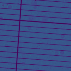
A microscope slide like the one above, whose divisions are a known distance apart, is used to perform the calculation.

First, a picture is taken of the ruler slide using the desired magnification. Next, the individual pixels between two divisions are counted. This is done using any editing software with a single-pixel brush size. Finally, the pixel size on the sensor plane of the imaging device must be known. Camera documentation should include this information.

Magnification is found by multiplying the counted number of pixels per division by the pixel size on the sensor plane and dividing by the actual distance of the divisions on the slide. An example calculation is performed below on a lens of approximately 10x magnification:

Calibration slide with 50 um divisions
Camera with 6.5 um pixel size
Counted 72 pixels per division

Magnification = (6.5*72)/50 = 9.36x

 

This semester, we collected 90 datasets of low resolution flatworm images to train the neural network on. The tomographic output is a high resolution and has a wide field of view. When training on the neural net is complete, we will be capable of single-shot reconstruction. Assuming the training is successful, we will write a paper on this research during the spring semester.

The foldscope project is proceeding more rapidly now that the flatworm project is nearing completion. We have prototyped multiple FPM-compatible assemblies using Legos and other material. Once our design is finalized, instructions for duplication will be posted to the blog along with images of the final product. We have experimented with apache cordova and other tools that will allow us to wirelessly control our LED array in sync with an iPhone camera using a simple app. The  ESP8266 dev board will be the key to wireless synchronization. The FPM app and any other software will be made available once complete so that any person with a foldscope, LED array, and cell phone can achieve single-shot Fourier reconstruction.

Our foldscope research is an extension of research completed this summer and during the 17/18 school year in Professor Ganapati’s lab. Using a neural network trained on low resolution input data and corresponding high resolution FPM reconstructions, we simultaneously optimize the illumination pattern and reconstruction algorithm.

The neural network identifies a single LED pattern to encode as much information about the sample as possible into one low resolution input image. By restricting our samples to a fixed type, we are able to significantly reduce the information requirements for reconstruction, making single-image reconstruction possible. The optimized reconstruction is also non-iterative, further improving temporal resolution.

For any given sample type, after training, we are able to generate a high resolution reconstruction from a single low resolution input image. We now aim to apply this technique with the foldscope to create an extremely low cost microscope capable of single image super-resolution microscopy.

Preprints:

“Optimal Physical Preprocessing for Example-Based Super-Resolution“

“Illumination Pattern Design with Deep Learning for Single-Shot Fourier Ptychographic Microscopy“

The foldscope is a paper microscope project designed to make quality microscopy portable and affordable. The bulk of the microscope is an origami-style paper assembly with sliders for manipulating the x, y, and z axes. The small lens can be affixed to a cellphone camera for easy imaging.

Foldscopes are useful anywhere lightweight, durable, and inexpensive scientific equipment is sought. They are used with paper centrifuges for low cost malaria detection, and in homes and schools to excite an interest in science on a budget.

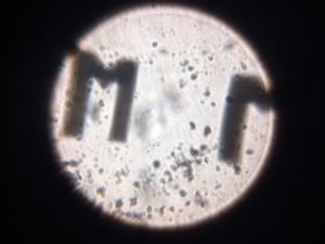
Our Foldscopes were easy to assemble with the provided instructions. We magnified a microscope slide and took a cell phone camera image while holding the slide up to a light.

The slide and lens were both somewhat dusty, and we could possibly have improved the focus with more careful adjustment. We decided, however, that this image would suffice as a proof of concept. Later, we built a temporary stand from Legos. The added stability improved overall image quality.

More information is available on the Foldscope website

And YouTube:

Manu Prakash: A 50-cent microscope that folds like origami

How to save 51 billion lives for 68 cents with simple Engineering