Author: Megan Strachan

We have written a program for the dome that randomly illuminates a fixed number of LEDs at random brightness. Multiplexed illumination is useful in Fourier ptychography because it reduces data collection time without sacrificing information (X). Our code generates several patterns of LEDs and takes one photo for each pattern.

Within the program, we define the number of LEDs to be lit, the number of bright field LEDs, and the number of total LEDs. Currently, we are only illuminating bright field LEDs during imaging. We define the total number of LEDs in anticipation of future imaging that does include the dark field images.

First, we determine the number of patterns to generate by dividing the number of LEDs in use by the number to be lit in each pattern (n). We generate a list of all possible LED indices and shuffle to randomize selection. Then, we assign n indices to each pattern. We pop each index off of the shuffled list, so no index is reused. We use numpy’s randint function to generate a brightness between 0 and 255 for each index.

The inbuilt LED dome commands do not provide for individual LED brightness assignment. Instead, we must reassign the brightness of the entire array before illuminating the desired index. In order to achieve LED patterns that contain many brightnesses, we reset the dome brightness before each LED is illuminated.

We collect and save an image before wiping the current pattern to begin illuminating the next. The section of code used to save the image is not included in the interest of brevity.

for i in range(numPatterns):
   for j in range(len(patterns[i])):

        #Get index of current LED
        light = patterns[i][j]

        #Get brightness of current LED
        intensity = brightness[i][j]

        #Set brightness and illuminate LED
        led_array.command(intensity)
        led_array.command(light)
   
   #Once the full pattern is illuminated, capture a photo  
   time.sleep(0.1)
   mmc.snapImage()

   #Clear the array in anticipation of the next pattern
   led_array.command('x')

Interfacing with the dome occurs extremely quickly. It is reasonable to reset the dome brightness and individually illuminate each LED because, even using this more tedious method, the entire pattern takes only a fraction of a second to display.

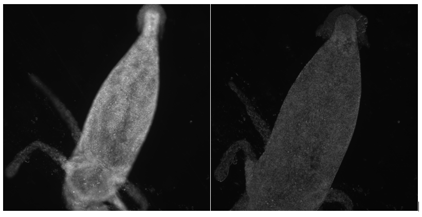
The LEDs in our dome are extremely bright, so we are able to significantly reduce the camera exposure time. Previously, we used an exposure of around 2 seconds for illumination by a single LED. For five LEDs of mixed brightness in our new array , an exposure of 0.15 seconds is perfectly sufficient. We have not yet determined the ideal exposure time for an image captured with only one fully bright LED illuminated.

Today, we mounted the new LED Dome to our microscope.

Our old array was mounted directly to the microscope stage, which made centering the sample over our objective lens inconvenient. We had to move samples into place by hand because using the stage controls to move samples also caused the LEDs to move and become uncentered.

In mounting our new array, we were careful to uncouple the LED array and the stage. We did this by reattaching the microscope’s condenser arm. This is the vertical piece that supported the microscope’s original illuminator lamp. First, we removed all of the old illuminating elements from the condenser to isolate the vertical condenser arm. Then we used a custom-made L-bracket to mount the optical breadboard plate parallel to the objective lens.

Our plate assembly is pictured below, with a zoomed in view of the L-bracket on the left and a view of the entire microscope, with the plate fixed to the condenser arm, on the right.

We made our L-bracket piece in the machine shop with help from J. Johnson, the machine shop supervisor. He helped us measure the space between screws and determine what diameter of screw was appropriate for each hole. He showed us how to drill holes of appropriate distance and size.

We used metal rods about 1 inch long to suspend the LED dome beneath the plate.

We adjusted the tightness of the screws until the assembly was level. Then we rewired the LED dome and tested some software written yesterday, which divides the brightfield LEDs into a fixed number of random patterns and displays them in turns. This test was successful.

 

 

Convolutional neural networks excel at visualization tasks, and are popular for tasks like single image super resolution (SR), where a high-resolution image is generated from a single low resolution input. SR is an ill-posed problem because for any one low resolution image, many high resolution interpretations are possible.

CNNs can learn the relationship between low-resolution images and their high-resolution counterparts. Generally, deeper neural networks are better able to generate these mappings. However, it is important that deep neural networks handle input data efficiently. Otherwise, they waste computational resources on information that will not cause the high-resolution output image to be more detailed or accurate.

Many CNNs developed for SR treat low and high frequency information from input images as equally necessary to computation. Low frequency information, which expresses gradual change in pixel intensity across the image, is easily extracted from low-resolution images. It can be forwarded more or less directly to the high-resolution output. High frequency information is an abrupt change in pixel intensity. It occurs in places of sharp intensity change, like edges. This is the detail that SR attempts to recover in order to generate a high-resolution output.

The network described in this paper, called RCAN (residual channel attention network),  adaptively learns the most useful features of input images. It uses a residual in residual structure to make the extremely deep network easier to train. Long and short skip connections allow the network to forward low frequency information directly toward the end of the architecture. The main portion of the network can therefore be dedicated to learning more useful high frequency information.

Above, a graphic from Zhang et al.’s paper illustrates the architecture of their network.

The RCAN network uses a post-upscaling strategy. Unlike other techniques, RCAN does not interpolate the low resolution input to the size of the output image before feeding it into the neural network. Preemptively enlarging the image increases the computational work that must be done and loses detail. Upscaling as a near-final step increases the efficiency of the network and preserves detail, resulting in more accurate outputs.

The residual in residual (RIR) structure used by RCAN pairs stacked residual blocks with a long skip connection. This allows the authors to have a very deep network (1,000+ layers) without making it impossible to train. They use a channel attention mechanism to emphasize network attention to the most useful information contained within the low resolution input. This most useful information is high frequency detail information, and is isolated by exploiting interdependencies between the network’s feature channels.

RCAN is shown by the authors to outperform other SR techniques, as shown below.

We are writing code that switches quickly between LED illumination patterns for rapid illumination.

Our usual illumination strategy saves individual LED coordinates and brightnesses in a .txt file. This text file is parsed by python code and passed into the serial port of the Arduino controlling our LED array. This method is slow because instead of illuminating the entire pattern at one time, LEDs are illuminated one by one.

When we are sequentially illuminating LEDs during data collection, our current strategy works well. We only need a single LED illuminated at any time, and we cannot image too quickly. Our images have a 2s exposure time because our LEDs are not very bright and they have a slow refresh rate. If we image too quickly, we experience banding.

Now, we want to be able to very quickly collect images under multiple specific illumination patterns. It is not efficient to individually illuminate LEDs when many are lit at the same time. Instead, we have written an Arduino program that assigns LED illumination patterns to a full array before illuminating. It takes milliseconds to switch back and forth between two full illumination patterns.

The desired LED illumination pattern is laid out in the style of the 8×8 example below, with individual array values representing the brightness of the corresponding LED.

 int image1[][8] ={
              {0,50,0,50,0,50,0,50},
              {0,70,0,70,0,70,0,70},
              {0,90,0,90,0,90,0,90},
              {0,110,0,110,0,110,0,110},
              {0,130,0,130,0,130,0,130},
              {0,150,0,150,0,150,0,150},
              {0,170,0,170,0,170,0,170},
              {0,190,0,190,0,190,0,190}
              };

This 8×8 array uses a brightness range from 0 to 255. Our full sized 32×32 array has a brightness range from 0 to 7.

We can create multiple illumination patterns and pass them to a function that illuminates the LED array accordingly. First, however, we must determine how best to translate the generated optical element into an Arduino array.

The neural network that generates the optimized optical element saves an npy file of illumination intensities, which are ordered in the same sequence as the LEDs are illuminated during data collection. We could open this npy file in python and examine it, then fill in the corresponding Arduino array by hand. We would prefer a quicker and less tedious solution; for example, we are looking to convert the provided npy file to a type more easily read by Arduino.

Our most recent project involves imaging small, multi cellular aquatic organisms called hydra. This organism is most notably known for its lack of aging since it is comprised mostly of regenerative stem cells. Our hydra are provided by a lab in Swarthmore’s biology department. We were given vials containing about 10 fixed regular and ‘inverted’ hydra. The inverted hydra have been sliced open and turned inside out, providing another perspective of the hydra for imaging. We were also given a pipette, a small glass dish with a hollow in the center, and a stack of cover slips to rest over the hydra.

As we began our imaging procedure, we quickly ran into problems. For instance, because we are imaging with an inverted microscope, there is a hole in the microscope stage over the objective lens. The dish we were given for imaging the hydra  was smaller than the hole in the stage, causing the dish to fall through and have no where to sit.  To fix this,  we acquired a larger dish, which did not have a center hollow.

We prepared hydra samples by pipetting one hydra onto the large dish and resting a cover slip on top. At first, this process appeared to work well. As imaging went on, however, we noticed that the body of the hydra seemed to expand and degrade. Below, we include the 1st and 137th images from one of our imaging datasets.

The hydra appears to have a different shape and density at the end of imaging than it did in the first image.

We brought our imaging results to our contact in the biology lab. We demonstrated our pipetting technique to show that the hydra were not being damaged during slide preparation. We mentioned that we had replaced the small dish with a larger one that had no center hollow because the small dish did not fit on the microscope stage.

The biologist explained that the dish hollow was an important feature that gave the hydra, a three-dimensional organism, space beneath the coverslip. When we applied the coverslip directly on top of our hydra, we were crushing it under the pressure of the cover slip. This caused the degradation we saw in our datasets.

He recommended building our own three-dimensional well for the hydra on a glass slide. By applying several layers of double sided tape on either side of the water droplet containing the hydra, we can raise the coverslip high enough that it does not crush the animal. This should prevent future sample degradation.

In the spring, we received two computers from the computer science department. Now that we are setting up the new lab in Singer Hall, we transferred control of the LED array microscope to one of the computers. Previously, data collection was run out of a very old, very slow laptop. The new computer should make work faster and more efficient.

First, we downloaded the python 2.7 distribution of Anaconda. Our lab prefers to run python programs in Spyder, a platform included in the Anaconda distribution. We use the built-in console and variable explorer to debug and monitor our progress. We also downloaded the Arduino IDE to control the LED array.

Our data collection program interfaces with both the Arduino and the PCO Edge camera. In order to run the program, we needed to install the camera software and move the files to a location where the python code could interact with them.

First, we tried to install the camera software using a USB that was given to us when the software was installed on the old laptop. This installation was unsuccessful. Instead, we downloaded camera software (pco.camware 4.07, 64 bit) from the PCO website (X).

Next, we downloaded micromanager. We added our PCO Edge to the micromanager environment using PCO’s micromanager guide (X). To test that micromanager was working correctly with the camera, we launched micromanager and watched a few seconds of the live camera feed.

Then we attempted to run python code that interfaces with the camera through micromanager. It did not work because the python code was not able to access the camera. We changed the python file configuration so that the code executed in the same folder as the mmgr_dal_PCO_Camera.dll file, which lets python and the camera interact through micromanager.

This solution is not ideal because our code executes and saves files in a folder very crowded with micromanager software. However, it does work. We are able to use our faster new computer to run all of the programs that were previously run on the laptop.

 

These notes are from the Google AI Blog post found here

Convolutional neural networks (CNNs) are usually created with a baseline model, then upgraded by scaling up certain dimensions of that model. This can include scaling up the width (adding more nodes to each layer), depth (adding more layers), or resolution (using a larger resolution of input images for training and evaluation), all for increased efficiency and accuracy of the CNN. Conventional methods scale each dimension independently and arbitrarily, and this requires a tedious manual tuning step in which training parameters are redefined to accommodate the new network size. The resulting upscaled CNN is often less accurate and less efficient than it might have been under more optimized scaling conditions.

In this paper, the authors propose a simple and effective scaling method that uniformly scales each dimension (depth, width, resolution of CNN) with a fixed set of scaling coefficients, depending on the computational capacity that can be afforded. A parameter sweep determines how to optimally scale depth, width, and input resolution to take advantage of available resources. These scaling coefficients are used to transform the base model. The resulting scaled model is called an EfficientNet. The models share a simple base image classification architecture that is scaled to generate different instances of the EfficientNet.

The EfficientNet models are capable of achieving state-of-the-art accuracy with many fewer parameters than competing networks. EfficientNet documentation and source code are available on GitHub (X).

 

 

Implementation (X)

References:

 

Blog by Victor Zhou (X)

The goal of this paper is to introduce the Deep Recursive Residual Network (DRRN), a type of CNN with the goal of providing a deep and effective model that uses many fewer parameters and has a higher performance than competing single image super-resolution (SISR) models.

The authors are motivated by recent models that achieve improved performance in super resolution reconstruction by adding many more layers (as many as 30) than previous designs (usually no more than 5). A pitfall of these deep models are their very large parameters. The described DRRN has significantly fewer parameters (2-14x less) while maintaining depth, with most DRRN models having as many as 52 layers.

Residual networks use an identity branch to retain the input to a residual block.  Then, the block only optimizes the residual mapping between the input and output instead of optimizing the mapping from input to output directly.

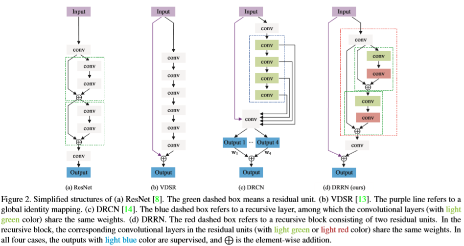
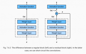
In the picture above (from the open source textbook ‘Dive into Deep Learning’), the difference between a regular (on the left) and residual block (right) is shown. The mapping output generated by the regular block, f(x), contains x more information than the residual block, and thus requires more computations. Residual blocks simplify the amount of input required and thus reduce computations.

The output of a SR model is anticipated to be highly similar to the input, so DRRN uses both residual learning. It employs both global residual learning, which connects the input and output images, and local residual learning, which ties the input and output of every few layers.

DRRN uses a recursive block of residual units that share weights to keep the model size small even though it is deep. Adding more depth (and consequently improving accuracy) can be done without adding more weight parameters. It uses a multi-path structure in the recursive block to avoid the vanishing/exploding gradients problem that appears in very deep models.

The figure above, taken from the paper by Tai et al., compares the basic structure of DRRN with other popular deep SR frameworks.

By combining global and local residual learning, the authors achieve visibly finer resolution than competing networks. Weight sharing in the recursive model allows them to deepen their network without requiring many parameters. Implementations of DRRN are available in tensorflow and pytorch in addition to the original caffe implementation (X).

The DRRN architecture may be very useful for our lab. Accurately and efficiently mapping low resolution images to corresponding high resolution images is a priority of our microscopy research. When comparing to a previous post describing the UNet, a different type of CNN, we found that while both are fast, highly effective networks, their purposes diverge. As stated earlier, DRRN models are designed for effective single-shot super-resolution, a central focus of our research, while Unet models are designed for image segmentation and multi-categorization. While this is a potential extension of our research, it appears that the DRRN model better fits the needs of our current research.

 

References

Y. Tai, J. Yang and X. Liu, “Image Super-Resolution via Deep Recursive Residual Network,” 2017 IEEE Conference on Computer Vision and Pattern Recognition (CVPR), Honolulu, HI, 2017, pp. 2790-2798.
doi: 10.1109/CVPR.2017.298

A. Zhang, Z.C. Lipton, M. Li and A.J. Smola, Dive into Deep Learning (X)

Tensorflow documentation offers useful introductory lessons on developing machine learning models for many uses.

First, we trained a basic classification network using the Fashion MNIST dataset. Like the canonical MNIST dataset, the Fashion MNIST consists of many thousands of 28×28 pixel images and associated image labels. This dataset pairs pictures of clothing items with one of nine class labels.

Below, a sample of images and associated labels is displayed. This plot is generated during the data inspection and preprocessing portion of the tutorial. To preprocess the data, pixel intensity values are scaled between 0 and 1 from the original 0-255.

Before the model can be trained, it must be built with an appropriate configuration of layers. Overcomplicated models are more sensitive to overfitting, so it is important to chose a sufficiently simple design.

## Set up the Model ##
model = keras.Sequential([

# Flatten the 28x28 input image into a 1d array of 784 pix
keras.layers.Flatten(input_shape=(28,28)),

# Create a dense/fully-connected layer with 128 nodes
keras.layers.Dense(128, activation=tf.nn.relu),

# Create a dense/fully-connected 'softmax' layer that returns 10 probability
# scores (one for each class) that sum to 1
keras.layers.Dense(10, activation=tf.nn.softmax)
])

The optimizer, loss function, and metrics of the model are chosen during the compile step. The optimizer (Adam, Stochastic gradient descent, etc.) defines the way that the model is updated .The loss function prioritizes minimization of different types of error. Metrics evaluate the successfulness of a step.

## Compile the model 

# Chose a loss function, optimizer, and metric(s)
model.compile(optimizer='adam',
             loss='sparse_categorical_crossentropy',
             metrics=['accuracy'])

Next, the model was trained on the training data using fit command.

model.fit(train_images, train_labels, epochs=5)

After training, the test data were used to evaluate the accuracy of the model.

test_loss, test_acc = model.evaluate(test_images, 
test_labels)

Finally, the model was used to predict classifications of the test dataset. Below is a plot of the output of my implementation of the model. Each image is displayed with the model’s prediction and confidence alongside the correct label. A bar plot of probabilities for each label is displayed next to the image.

It is notable that these results are not identical to those in the tensorflow documentation, but are very similar. The model builds its own association between the training data and corresponding tags, and may learn slightly different relationships each time it is built and trained.

Our commented implementation of the tensorflow walkthrough may be viewed here.

 

We also completed an example of sentiment classification in text (positive or negative) and a deep convolutional general adversarial network (DCGAN)designed to generate ‘written’ numbers in the style of the classic MNIST dataset, both using walkthroughs in the tensorflow documentation pages.

In the case of the DCGAN, we were able to observe improvement from patchy white noise to moderately resolved shapes. However, our personal computers lack the computational power to quickly train a model of this type, and we have not yet completed the prescribed 50 epochs.

 

The same Fashion MNIST example is available for other deep learning frameworks, including pytorch. Progress on these implementations has temporarily stalled because documentation is more limited than for tensorflow and because Google colab does not easily support all of the libraries used in pytorch examples.