
Tensorflow documentation offers useful introductory lessons on developing machine learning models for many uses.
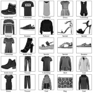
First, we trained a basic classification network using the Fashion MNIST dataset. Like the canonical MNIST dataset, the Fashion MNIST consists of many thousands of 28×28 pixel images and associated image labels. This dataset pairs pictures of clothing items with one of nine class labels.
Below, a sample of images and associated labels is displayed. This plot is generated during the data inspection and preprocessing portion of the tutorial. To preprocess the data, pixel intensity values are scaled between 0 and 1 from the original 0-255.
Before the model can be trained, it must be built with an appropriate configuration of layers. Overcomplicated models are more sensitive to overfitting, so it is important to chose a sufficiently simple design.
## Set up the Model ##
model = keras.Sequential([

# Flatten the 28x28 input image into a 1d array of 784 pix
keras.layers.Flatten(input_shape=(28,28)),

# Create a dense/fully-connected layer with 128 nodes
keras.layers.Dense(128, activation=tf.nn.relu),

# Create a dense/fully-connected 'softmax' layer that returns 10 probability
# scores (one for each class) that sum to 1
keras.layers.Dense(10, activation=tf.nn.softmax)
])
The optimizer, loss function, and metrics of the model are chosen during the compile step. The optimizer (Adam, Stochastic gradient descent, etc.) defines the way that the model is updated .The loss function prioritizes minimization of different types of error. Metrics evaluate the successfulness of a step.
## Compile the model

# Chose a loss function, optimizer, and metric(s)
model.compile(optimizer='adam',
             loss='sparse_categorical_crossentropy',
             metrics=['accuracy'])
Next, the model was trained on the training data using fit command.
model.fit(train_images, train_labels, epochs=5)
After training, the test data were used to evaluate the accuracy of the model.
test_loss, test_acc = model.evaluate(test_images,
test_labels)
Finally, the model was used to predict classifications of the test dataset. Below is a plot of the output of my implementation of the model. Each image is displayed with the model’s prediction and confidence alongside the correct label. A bar plot of probabilities for each label is displayed next to the image.
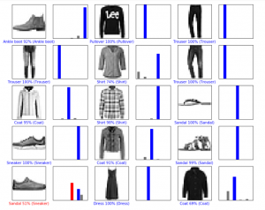
It is notable that these results are not identical to those in the tensorflow documentation, but are very similar. The model builds its own association between the training data and corresponding tags, and may learn slightly different relationships each time it is built and trained.
Our commented implementation of the tensorflow walkthrough may be viewed here.
We also completed an example of sentiment classification in text (positive or negative) and a deep convolutional general adversarial network (DCGAN)designed to generate ‘written’ numbers in the style of the classic MNIST dataset, both using walkthroughs in the tensorflow documentation pages.
In the case of the DCGAN, we were able to observe improvement from patchy white noise to moderately resolved shapes. However, our personal computers lack the computational power to quickly train a model of this type, and we have not yet completed the prescribed 50 epochs.
The same Fashion MNIST example is available for other deep learning frameworks, including pytorch. Progress on these implementations has temporarily stalled because documentation is more limited than for tensorflow and because Google colab does not easily support all of the libraries used in pytorch examples.