Convolutional Neural Networks:
Convolutional neural networks (CNNs) are a type of deep learning neural network specifically geared towards image recognition. CNNs are most commonly used with categorical classification problems. The application of CNNs are widespread, from recognition of cars on roads or faces in photos to teaching a computer to play a video game with an ability that much surpasses human skill. One application discussed in more detail in this post is the U-net CNN, which is designed for biomedical imaging. CNNs often use dense, fully connected networks, which like many neural networks makes it prone to the common problem of overfitting. For most types of neural networks, overfitting is fixed by various forms of regularization, such as dropout or weight regularization. CNNs instead approach the problem of overfitting by breaking down complex patterns in images into smaller and simpler patterns. It accomplishes this using methods like filtering and pooling, which will be addressed in this post.
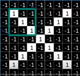
CNNs start by taking a set of training images as input. In each image, pixels may contain a certain pattern or be absent of that pattern. For each pixel, if the pattern is present, it is labeled as a 1, or a -1 if it is absent of that pattern. For instance, if you have an image of a handwritten single digit number, the place where the writing is present will be labeled as 1, everywhere else as -1. Take a look at Brandon Rohrer’s image from the Youtube video “How Convolutional Neural Networks Work” below for an example.
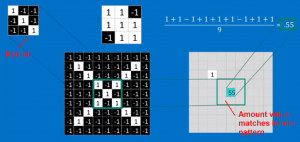
These images are given as input to a convolutional layer. In a convolutional layer, the image undergoes a process known as filtering. In filtering, you take a feature pattern, known as a kernel, and compare it to little pieces of the whole image. The size of the feature pattern is known as its kernel size. By multiplying each matching pixel together (matrix multiplication) and summing these values up, you get a value that represents how closely the feature pattern matches the little piece of an image you are looking at. A more positive value is a closer match, a negative value means there is little to no match. Then you move the feature pattern over to the next little piece of the image and perform this procedure again. The movement of the kernel across the image is known as striding, and the stride is the step size of the kernel when walking across the image. Typical strides tend to be 1 or 2. The final image after all the values are recorded is called the convolved feature. In the Rohrer’s video example below, a kernel of 3×3 kernel size is being used for filtering. The little piece that is being compared shows a match of .55.
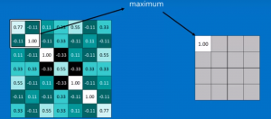
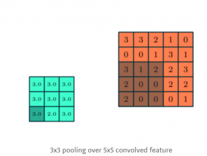
After filtering, all of these images are stacked together by the convolutional layer before the process of pooling. Pooling is when you shrink the image stack by looking at little pieces of the convolved image at a time and selecting the maximum value. This can be better understood by the Rohrer’s youtube image below. Notice how in the selected 2×2 window, the maximum value in this convolved image is 1.00.
All of these maximum values are put together into a new image that is much smaller than the original convolved image. This is a key part of the CNN method of breaking down complex and bigger patterns in images into smaller and simpler patterns, which all helps decrease the chances of overfitting. Another image from Sumit Saha’s article ” A comprehensive Guide to CNNs–the EL15 Way” is shown below.
Finally, in many CNNs, there is a layer known as the rectified linear unit (reLu) layer. In this layer, any negative maximum values in the pooled image is change to a 0 in a process called normalization. This ensures that all maximum values in the pooled images are between the range of 0-1, with 1 being a complete pattern match and 0 being no pattern match at all.
All of these convolution layers , pooling layers, and reLu layers get stacked up in a CNN so the output of one becomes the input of the next. Deep stacking is when the layers get stacked several times. Each time through, the image gets smaller (through pooling) and more and more simplified (through filtering). At the very end is a fully connected layer which is able to classify each simplified image into the correct category.
U-Net CNNs for Biomedical Image Segmentation:
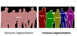
U-net is a type of CNN created for biomedical image segmentation. In image segmentation, a digital image is split into several segments or groups of pixels, with each pixel in an image assigned a specific categorical label. Image segmentation is especially useful for identifying objects and boundaries, like lines and curves. There are two types of image segmentation: semantic and instance image segmentation. Semantic is to label each pixel of an image as a certain category or class. Instance segmentation is slightly more advanced, where the computer is able classify each new occurrence of a class separately.
In a U-net CNN, the training data is made much larger by breaking images down into patches or groups of pixels. This way, the number of training data is increased from the number of training images given as input to the number of training patches.
A U-net CNN is named for its U-shaped network architecture, in which the left half is a contracting path that is nearly symmetric to the right expansive path. The contracting path is more of a typical CNN, consisting of two convolution layers with a 3×3 kernel size, each followed by a rectified linear unit (ReLU) layer and a pooling layer with window size of 2×2 and stride 2. The expansive path consists of an upsampling of the images, which replaces pooling layers and helps to increase the resolution of the output. This is followed by a 2×2 convolution (“up-convolution”) and two 3×3 convolution layers, each fol-
lowed by a ReLU layer. In total the network has 23 layers.
The pieces of code below are snippets of an example U-net implementation in tensorFlow on GitHub by Mo Kweon. Like always, the necessary libraries are imported, including libraries already discussed like pandas.
import time
import os
import pandas as pd
import tensorflow as tf
In this code snippet, the kernel size and stride of a convolution layer is being defined.
    return tf.layers.conv2d_transpose(
        tensor,
        filters=n_filter,
        kernel_size=2,
        strides=2,
        kernel_regularizer=tf.contrib.layers.l2_regularizer(flags.reg),
        name="upsample_{}".format(name))
In the code below, you can see the pooling layers being replaced by upsampling for a higher resolution output.
up6 = upconv_concat(conv5, conv4, 64, flags, name=6
   conv6 = conv_conv_pool(up6, [64, 64], training, flags, name=6, pool=False)
Like with keras , every neural network needs to have a defined loss function and optimizer.
loss = -IOU_(y_pred, y_true)
global_step = tf.train.get_or_create_global_step()

optim = tf.train.AdamOptimizer()
return optim.minimize(loss, global_step=global_step)
Finally, one more snippet of code below shows that for every epoch (round of training), a data sample of some batch_size is trained.
for epoch in range(flags.epochs):
        for step in range(0, n_train, flags.batch_size):
References:
https://towardsdatascience.com/types-of-convolutions-in-deep-learning-717013397f4d
https://towardsdatascience.com/a-comprehensive-guide-to-convolutional-neural-networks-the-eli5-way-3bd2b1164a53
Youtube: How Convolutional Neural Networks Work
https://en.wikipedia.org/wiki/Convolutional_neural_network
https://github.com/kkweon/UNet-in-Tensorflow/blob/master/train.py
O. Ronneberger, P. Fischer, and T. Brox. “U-Net: Convolutional Networks for Biomedical Image Segmentation”. University of Freiburg, Germany. 2015.