Month: June 2019

Convolutional neural networks excel at visualization tasks, and are popular for tasks like single image super resolution (SR), where a high-resolution image is generated from a single low resolution input. SR is an ill-posed problem because for any one low resolution image, many high resolution interpretations are possible.

CNNs can learn the relationship between low-resolution images and their high-resolution counterparts. Generally, deeper neural networks are better able to generate these mappings. However, it is important that deep neural networks handle input data efficiently. Otherwise, they waste computational resources on information that will not cause the high-resolution output image to be more detailed or accurate.

Many CNNs developed for SR treat low and high frequency information from input images as equally necessary to computation. Low frequency information, which expresses gradual change in pixel intensity across the image, is easily extracted from low-resolution images. It can be forwarded more or less directly to the high-resolution output. High frequency information is an abrupt change in pixel intensity. It occurs in places of sharp intensity change, like edges. This is the detail that SR attempts to recover in order to generate a high-resolution output.

The network described in this paper, called RCAN (residual channel attention network),  adaptively learns the most useful features of input images. It uses a residual in residual structure to make the extremely deep network easier to train. Long and short skip connections allow the network to forward low frequency information directly toward the end of the architecture. The main portion of the network can therefore be dedicated to learning more useful high frequency information.

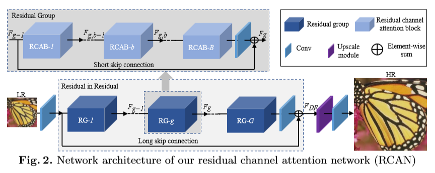
Above, a graphic from Zhang et al.’s paper illustrates the architecture of their network.

The RCAN network uses a post-upscaling strategy. Unlike other techniques, RCAN does not interpolate the low resolution input to the size of the output image before feeding it into the neural network. Preemptively enlarging the image increases the computational work that must be done and loses detail. Upscaling as a near-final step increases the efficiency of the network and preserves detail, resulting in more accurate outputs.

The residual in residual (RIR) structure used by RCAN pairs stacked residual blocks with a long skip connection. This allows the authors to have a very deep network (1,000+ layers) without making it impossible to train. They use a channel attention mechanism to emphasize network attention to the most useful information contained within the low resolution input. This most useful information is high frequency detail information, and is isolated by exploiting interdependencies between the network’s feature channels.

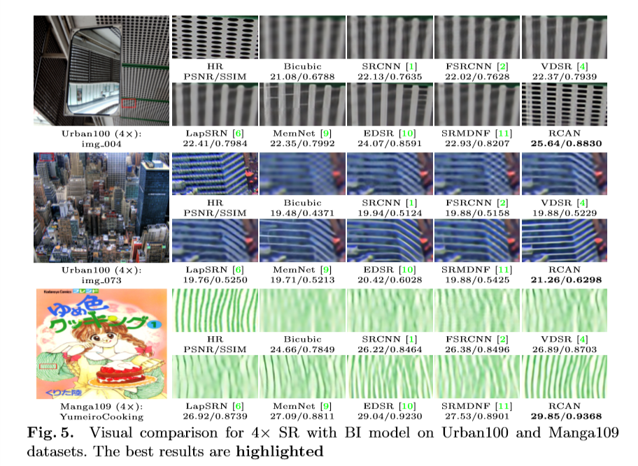
RCAN is shown by the authors to outperform other SR techniques, as shown below.

We are writing code that switches quickly between LED illumination patterns for rapid illumination.

Our usual illumination strategy saves individual LED coordinates and brightnesses in a .txt file. This text file is parsed by python code and passed into the serial port of the Arduino controlling our LED array. This method is slow because instead of illuminating the entire pattern at one time, LEDs are illuminated one by one.

When we are sequentially illuminating LEDs during data collection, our current strategy works well. We only need a single LED illuminated at any time, and we cannot image too quickly. Our images have a 2s exposure time because our LEDs are not very bright and they have a slow refresh rate. If we image too quickly, we experience banding.

Now, we want to be able to very quickly collect images under multiple specific illumination patterns. It is not efficient to individually illuminate LEDs when many are lit at the same time. Instead, we have written an Arduino program that assigns LED illumination patterns to a full array before illuminating. It takes milliseconds to switch back and forth between two full illumination patterns.

The desired LED illumination pattern is laid out in the style of the 8×8 example below, with individual array values representing the brightness of the corresponding LED.

 int image1[][8] ={
              {0,50,0,50,0,50,0,50},
              {0,70,0,70,0,70,0,70},
              {0,90,0,90,0,90,0,90},
              {0,110,0,110,0,110,0,110},
              {0,130,0,130,0,130,0,130},
              {0,150,0,150,0,150,0,150},
              {0,170,0,170,0,170,0,170},
              {0,190,0,190,0,190,0,190}
              };

This 8×8 array uses a brightness range from 0 to 255. Our full sized 32×32 array has a brightness range from 0 to 7.

We can create multiple illumination patterns and pass them to a function that illuminates the LED array accordingly. First, however, we must determine how best to translate the generated optical element into an Arduino array.

The neural network that generates the optimized optical element saves an npy file of illumination intensities, which are ordered in the same sequence as the LEDs are illuminated during data collection. We could open this npy file in python and examine it, then fill in the corresponding Arduino array by hand. We would prefer a quicker and less tedious solution; for example, we are looking to convert the provided npy file to a type more easily read by Arduino.

As we image and pre-process the hydra data, we have continued to encounter unexpected problems, leading us to make changes to our imaging procedure in order to best optimize the output of our data.

The first issue we encountered was the fact that the hydra were being flattened by the pressure of the cover slip while imaging was taking place. This caused the slow degradation of the hydra, causing major differences between image 0 and image 68 (see image below).

Differences between each of the 69 images in each stack, other than the change of position of the light source due to the each illuminated LED, are problematic and result in poor training data for the neural network.  The lab group solved this problem by stacking up double-sided tape on the slides with the cover slip sitting on top, allowing for a 3-dimensional gap for the hydra to rest in during imaging.

While the hydra itself are now better preserved during imaging, we have since come across additional imaging problems.  We tried running our shift-add algorithm,  which takes the low resolution stack of images and analyzes the image at different z-distances (depths), producing different three-dimensional “slices” of the image. However, we found that the resulting image slices were completely saturated with light, producing the yellow image below.

The lab group quickly realized that stray light from the lab room was saturating the images in too much light. In order to eliminate stray light, it is necessary to image either in a dark room or with a cover completely over the FP microscope. The lab group chose to use a large cardboard box as a cover for the microscope and camera. We took more data, ran the shift-add algorithm, and were successfully able to produce image slices of the hydra. Below is a look at an example of an original low resolution image of a hydra and a couple of its resulting slices from the shift-add algorithm.

The final problem, and so far one of the most difficult to solve, is the subtle movements of the water surrounding the hydra in the slide. These small movements of the water, caused by factors such as tiny shaking of the building, so small that they are nearly undetectable, cause the hydra to move ever so slightly in the flowing water. This results in a visual and problematic shift between image 0 and image 68 in a stack (example shown below), producing poor training data for the neural network.

The ideal way to solve this problem is to use a specially designed optical table, which corrects for minute movements and shakes such as these. However, the lab currently is not equipped with an optical table, so alternative attempts at a solution have been made. Currently the lab group is using a tray with small dishes for imaging. We figure that with smaller dishes, the water has no place to move and expand, whereas with the taped slide method, there were empty pockets of space for the water to flow into. The potential drawback with this method is the tray is made of thicker plastic compared to the glass slide, which could possibly produce less clear images.

After fixing the issue of keeping the hydras from being flattened by the cover slip, we began collecting low-resolution images of the hydras to start running algorithms for reconstructing a high-resolution image.

We chose a sample data set with one stack of images and ran the Generatescript.py code. By executing the sh file that it created, we ran into a problem in which no high resolution image was generated. To see if the problem lay with the program or the images, we tried running the code with a flatworm data set imaged last summer. This succeeded in producing the high resolution image, confirming that the issue relates to our hydra data somehow.

Currently we suspect that the one stack of data is not sufficient for the pre-processing procedure, so we are currently trying with a five-stack hydra data set for the GenerateScript.py. Once the program stops running, we will see if this is in fact the source of the problem or not.

Our most recent project involves imaging small, multi cellular aquatic organisms called hydra. This organism is most notably known for its lack of aging since it is comprised mostly of regenerative stem cells. Our hydra are provided by a lab in Swarthmore’s biology department. We were given vials containing about 10 fixed regular and ‘inverted’ hydra. The inverted hydra have been sliced open and turned inside out, providing another perspective of the hydra for imaging. We were also given a pipette, a small glass dish with a hollow in the center, and a stack of cover slips to rest over the hydra.

As we began our imaging procedure, we quickly ran into problems. For instance, because we are imaging with an inverted microscope, there is a hole in the microscope stage over the objective lens. The dish we were given for imaging the hydra  was smaller than the hole in the stage, causing the dish to fall through and have no where to sit.  To fix this,  we acquired a larger dish, which did not have a center hollow.

We prepared hydra samples by pipetting one hydra onto the large dish and resting a cover slip on top. At first, this process appeared to work well. As imaging went on, however, we noticed that the body of the hydra seemed to expand and degrade. Below, we include the 1st and 137th images from one of our imaging datasets.

The hydra appears to have a different shape and density at the end of imaging than it did in the first image.

We brought our imaging results to our contact in the biology lab. We demonstrated our pipetting technique to show that the hydra were not being damaged during slide preparation. We mentioned that we had replaced the small dish with a larger one that had no center hollow because the small dish did not fit on the microscope stage.

The biologist explained that the dish hollow was an important feature that gave the hydra, a three-dimensional organism, space beneath the coverslip. When we applied the coverslip directly on top of our hydra, we were crushing it under the pressure of the cover slip. This caused the degradation we saw in our datasets.

He recommended building our own three-dimensional well for the hydra on a glass slide. By applying several layers of double sided tape on either side of the water droplet containing the hydra, we can raise the coverslip high enough that it does not crush the animal. This should prevent future sample degradation.

Now that all the computers are set up except for the one with the monitor that will be using for data processing, we started collecting  low resolution image stacks from the hydras we received from Swarthmore’s biology department.

By placing the hydra into a dish and stabilizing it with a square plastic cover, we are able to observe the hydra under the Fourier Ptychographic microscope and collect photos using the camera.

We took photos with three different diameters of the LED matrix, specifically 9, 11 and 13. By lighting up different ranges of LED lights, we were able to create three low resolution data sets with 1 low resolution stack per diameter. After taking these datasets, we will decided that the 10x magnification is best if we want to be able to image the entire hydra rather than a part of that hydra.

Shift-add algorithms and the iterative reconstruction algorithm will be implemented once the computer with the algorithms is set up.

In the spring, we received two computers from the computer science department. Now that we are setting up the new lab in Singer Hall, we transferred control of the LED array microscope to one of the computers. Previously, data collection was run out of a very old, very slow laptop. The new computer should make work faster and more efficient.

First, we downloaded the python 2.7 distribution of Anaconda. Our lab prefers to run python programs in Spyder, a platform included in the Anaconda distribution. We use the built-in console and variable explorer to debug and monitor our progress. We also downloaded the Arduino IDE to control the LED array.

Our data collection program interfaces with both the Arduino and the PCO Edge camera. In order to run the program, we needed to install the camera software and move the files to a location where the python code could interact with them.

First, we tried to install the camera software using a USB that was given to us when the software was installed on the old laptop. This installation was unsuccessful. Instead, we downloaded camera software (pco.camware 4.07, 64 bit) from the PCO website (X).

Next, we downloaded micromanager. We added our PCO Edge to the micromanager environment using PCO’s micromanager guide (X). To test that micromanager was working correctly with the camera, we launched micromanager and watched a few seconds of the live camera feed.

Then we attempted to run python code that interfaces with the camera through micromanager. It did not work because the python code was not able to access the camera. We changed the python file configuration so that the code executed in the same folder as the mmgr_dal_PCO_Camera.dll file, which lets python and the camera interact through micromanager.

This solution is not ideal because our code executes and saves files in a folder very crowded with micromanager software. However, it does work. We are able to use our faster new computer to run all of the programs that were previously run on the laptop.

 

To assemble the Fourier Ptychographic mircosope (FPM), we first rewired the Arduino where it had become disconnected during storage and restored the input and power connections to the array before mounting it over the microscope objective. Fortunately, the wiring for the Arduino connected to the LED array was mostly already set up, saving a large portion of time.

The pco camera was refitted with our c mount adapter and attached to the microscope. Power and usb cables were used to connect the camera to our laptop and the outlet. The 10x, 20x, and 40x objectives were also attached into place just under the stage.

We first tested the functionality of the LED array using our LEDPlayground Arduino file, which illuminates a small section of the LED array. After successfully illuminating the array, we fully tested our imaging procedure on the reassembled microscope.

The test run was performed using a calibration slide, which consists of grids and numbers for points of reference when focusing. We chose a diameter of 9 LEDs and collected a total of 69 images of the calibration slide. The resulting image stack appeared as expected, with small variations present between images as the illumination angle shifted slightly.

The successful test run confirms that  the microscope has been reassembled correctly and is ready for use collecting data sets of unstained, fixed hydra samples.

 

These notes are from the Google AI Blog post found here

Convolutional neural networks (CNNs) are usually created with a baseline model, then upgraded by scaling up certain dimensions of that model. This can include scaling up the width (adding more nodes to each layer), depth (adding more layers), or resolution (using a larger resolution of input images for training and evaluation), all for increased efficiency and accuracy of the CNN. Conventional methods scale each dimension independently and arbitrarily, and this requires a tedious manual tuning step in which training parameters are redefined to accommodate the new network size. The resulting upscaled CNN is often less accurate and less efficient than it might have been under more optimized scaling conditions.

In this paper, the authors propose a simple and effective scaling method that uniformly scales each dimension (depth, width, resolution of CNN) with a fixed set of scaling coefficients, depending on the computational capacity that can be afforded. A parameter sweep determines how to optimally scale depth, width, and input resolution to take advantage of available resources. These scaling coefficients are used to transform the base model. The resulting scaled model is called an EfficientNet. The models share a simple base image classification architecture that is scaled to generate different instances of the EfficientNet.

The EfficientNet models are capable of achieving state-of-the-art accuracy with many fewer parameters than competing networks. EfficientNet documentation and source code are available on GitHub (X).

The paper focuses on illumination angle self-calibration for Fourier ptychographic microscopy (FPM).  However, there appears to be errors in FPM due to shifts or rotations of the LED array, source instabilities, nonplanar illuminator arrangements, or sample-induced aberrations. The paper proposes  a two-pronged-angle self-calibration method that uses both preprocessing (brightfield calibration) and iterative joint estimation (spectral correlation calibration) that is quicker and more robust to system changes than state- of-the-art calibration methods.

For the Brightfield calibration, the following algorithm is used to perform the task.

For Spectral Correlation Calibration, we can see from the figure below that cost function is lower when both BC and SC are implemented.

 

References: 

R. Eckert, Z.F. Phillips,L.Waller.”Efficient illumination angle self-calibration in Fourier ptychography”, 2018 Optical Society of America