Potential Super Resolution Algorithms for Fluorescence Microscopy: SIM and PSF

Currently in Ganapati’s lab, we are using Fourier Ptychographic Microscopy (FPM) to image biological samples. This type of microscopy  involves using an LED dome to illuminate the sample in many different illumination angles, allowing for increased image information of the sample with both dark field and bright field images. However, we have come across some challenges with FPM  when using thick or transparent biological samples.

A different type of microscopy that is better suited for thick biological samples is fluorescence microscopy. In florescence microscopy, a sample is stained with various fluorophore dyes, with each dye attaching to different organic or mineral components of the sample. The stained sample is then bathed in intense light, causing the specimen to fluoresce. Because the specimen is now labeled with dyes, it is much easier to visually distinguish different layers of the sample in the image.

There are multiple types of super resolution algorithms that can be used for fourescence microscopy, but two in particular that this lab is interested in are structured light microscopy (SIM) and the point spread function (PSF).

Structured Light Microscopy (SIM):

SIM uses the idea of Moiré‘s Law to aid in super resolution.  Moiré‘s Law can be seen on certain images or on television, producing a wavy pattern. This  Moiré pattern occurs when an object that is being photographed contains some sort of pattern, like stripes or dots, that exceed the resolution of the sensor. This is the same idea as “beats” in sound, and happens as a result of the interference of waves.
SIM technology takes advantage of the Moiré effect in order to extract higher resolution information from the image. In SIM, a striped or dotted illumination pattern is placed just before the sample. This pattern excites the sample, causing it to fluoresce. The interference of the fluorescence emission and excitation waves creates a Moiré pattern, which can be used and interpreted by a computer algorithm to find more spatial information about the image. This in turn allows for the enhancement of the resolution of the image .
A Github repository for a SIM super resolution algorithm can be found here:


Point Spread Function (PSF):

When you are viewing a microscopic fluorescent object under a microscope, the diffraction of light from the emitted fluorescence will cause the object to appear blurred. This blurring, which occurs in both the lateral and depth direction of the object, is known as the point spread function (PSF). PSF tend to have worse blurring in the depth direction, since microscopes tend to have worse resolution in that direction.

In order to minimize the effects of the PSF and reduce blurring, some modifications to the hardware of the microscope can be made, such as having a shorter wavelength of illumination light and  increasing the numerical aperture of the objective lens. On the software side, computer algorithms can “undo” the blurring  caused by the PSF by performing computational deconvolutions, which reverse the effects of the PSF and enhance the resolution of the image.

A Github repository for a PSF super resolution algorithm can be found here: https://github.com/FerreolS/tipi4icy

Resources:

A. Lal, C. Shan, and P. Xi . “Structured Ilumination Image Reconstruction Algorithm.” Department of  Biomedical Engineering,  Peking University. IEEE Journal. 4.(2016).

K. Sring and M. Davidson. “Introduction to Fluorescence Microscopy.” MicroscopyU.

“A Beginners Guide to the Point Spread Function”. Zeiss Microscopy.

A. Lavdas “Structured Illumination Microscopy–An Introduction.” Bitesizebio.com

N. Mansurov. “What is Moiré?” PhotographyLife.com (2012).

Advantages and Familiarization with the new LED Dome

The Fourier Ptychographic Microscopy (FPM) so far in Ganapati’s lab has been performed with a flat 32×32 LED array.  With a flat array, you can light up one LED at a time to acquire different illumination angles for imaging. However, there are many disadvantages to the current flat LED array set-up. For example, one major issue  regarding the flat LED array is that it is programmed by Arduino, which does not contain memory. When we tried to reprogram the array to light up random multiplexed patterns of LEDs rather than one LED at a time (a change that could greatly reduce data acquisition time), we were unable to do so because the Arduino could not store information on the location of the LED coordinates. In addition, the flat LED is not very bright and contains smaller illumination angles, producing low resolution images that contain less intensity information and therefore decreases the space-bandwidth product (SBP) of the FPM reconstructed images.

By replacing the flat LED array with an LED dome purchased from Spectral Coded Illumination (Sci), many improvements could be made to our current FPM procedure.  We can easily program the dome to produce random multiplexed patterns of LEDs because the LED can be programmed directly through Python, a much more robust and easy-to-use software than Arduino that can easily store information. In addition, each LED is assigned a specific number rather than a x-y coordinate position, making it easier to write programs that access certain LEDs.

Because of the sloped sides of the array, which produces a dome shape, the LED dome can produce much higher angles for dark field illumination, allowing for increased intensity information of images and thus increasing the SBP of the reconstructed high resolution image. In addition, the LED dome is much brighter than the flat LED array, also contributing to higher quality images and better data for reconstruction. Finally, the dome is programmed to sweep through and illuminate LEDs  at a much faster rate than the flat array, significantly reducing data acquisition time.

Once we received the LED dome, we proceeded to download the necessary programs and become familiarized with the various commands for the dome. For instance, the command ‘bf’ illuminates only the brightfield LEDs, which are the LEDs located at low illumination angles and located directly above in sample in the flat roof of the dome. Other examples of commands are shown but not limited to the list below:

‘df’    illuminates only the dark field LEDs.

‘ff’     illuminates all LEDs in the array

‘sb.[r].[g].[b]’   sets the brightness of the array

‘scf’       lights up each LED in the array individually. Takes less than 1 minute to fully scan.

‘x’ clears the array

In the next few days we plan to learn more about setting up the hardware trigger modes for direct communication between the PCO camera and dome. We also plan to design and create a way to mount the LED dome onto the microscope so that we can allow for an automated stage. Currently with our flat LED array, we have the array attached to the stage, confining the lab group to manually moving the slides with our hands rather than having a more precise automated stage system.


Changes in Hydra Imaging Procedure

As we image and pre-process the hydra data, we have continued to encounter unexpected problems, leading us to make changes to our imaging procedure in order to best optimize the output of our data.

The first issue we encountered was the fact that the hydra were being flattened by the pressure of the cover slip while imaging was taking place. This caused the slow degradation of the hydra, causing major differences between image 0 and image 68 (see image below).

Differences between each of the 69 images in each stack, other than the change of position of the light source due to the each illuminated LED, are problematic and result in poor training data for the neural network.  The lab group solved this problem by stacking up double-sided tape on the slides with the cover slip sitting on top, allowing for a 3-dimensional gap for the hydra to rest in during imaging.

While the hydra itself are now better preserved during imaging, we have since come across additional imaging problems.  We tried running our shift-add algorithm,  which takes the low resolution stack of images and analyzes the image at different z-distances (depths), producing different three-dimensional “slices” of the image. However, we found that the resulting image slices were completely saturated with light, producing the yellow image below.

The lab group quickly realized that stray light from the lab room was saturating the images in too much light. In order to eliminate stray light, it is necessary to image either in a dark room or with a cover completely over the FP microscope. The lab group chose to use a large cardboard box as a cover for the microscope and camera. We took more data, ran the shift-add algorithm, and were successfully able to produce image slices of the hydra. Below is a look at an example of an original low resolution image of a hydra and a couple of its resulting slices from the shift-add algorithm.

The final problem, and so far one of the most difficult to solve, is the subtle movements of the water surrounding the hydra in the slide. These small movements of the water, caused by factors such as tiny shaking of the building, so small that they are nearly undetectable, cause the hydra to move ever so slightly in the flowing water. This results in a visual and problematic shift between image 0 and image 68 in a stack (example shown below), producing poor training data for the neural network.

The ideal way to solve this problem is to use a specially designed optical table, which corrects for minute movements and shakes such as these. However, the lab currently is not equipped with an optical table, so alternative attempts at a solution have been made. Currently the lab group is using a tray with small dishes for imaging. We figure that with smaller dishes, the water has no place to move and expand, whereas with the taped slide method, there were empty pockets of space for the water to flow into. The potential drawback with this method is the tray is made of thicker plastic compared to the glass slide, which could possibly produce less clear images.

Assembling the Fourier Ptychographic Microscope and Running a Test Trial

To assemble the Fourier Ptychographic mircosope (FPM), we first rewired the Arduino where it had become disconnected during storage and restored the input and power connections to the array before mounting it over the microscope objective. Fortunately, the wiring for the Arduino connected to the LED array was mostly already set up, saving a large portion of time.

The pco camera was refitted with our c mount adapter and attached to the microscope. Power and usb cables were used to connect the camera to our laptop and the outlet. The 10x, 20x, and 40x objectives were also attached into place just under the stage.

We first tested the functionality of the LED array using our LEDPlayground Arduino file, which illuminates a small section of the LED array. After successfully illuminating the array, we fully tested our imaging procedure on the reassembled microscope.

The test run was performed using a calibration slide, which consists of grids and numbers for points of reference when focusing. We chose a diameter of 9 LEDs and collected a total of 69 images of the calibration slide. The resulting image stack appeared as expected, with small variations present between images as the illumination angle shifted slightly.

The successful test run confirms that  the microscope has been reassembled correctly and is ready for use collecting data sets of unstained, fixed hydra samples.


Notes on “Low-Cost, Sub-Micron Resolution, Wide-Field Computational Microscopy using Opensource Hardware” by T. Aidukas, R. Eckert, A. Harvey, L.Waller, and P. Konda

There is a heavy need for low-cost, portable microscopes for medical purposes and disease prevention in communities with limited resources. Attempts at microscopy suited for these communities have previously resulted in images with a poor space bandwidth product (SBP). Unfortunately, a high SBP is essential for accurate identification of diseases or targeted cells in medical diagnosis. SBP can be improved with expensive equipment such as automated stages for mechanical scanning and a high quality lens, but these costly materials are not feasible for resource-limited communities.

This paper by T. Aidukas, R. Eckert, A. Harvey, L. Waller, and P. Konda proposes a low-cost, portable microscope with a high SBP using a 3D printed Fourier Ptychographic microscope (FPM) equipped with an LED array and a Raspberry Pi computer board and camera. Using this setup,  multiple LR images are taken by the Raspberry Pi camera lens using  oblique illumination angles from the LED array. Using the Raspberry Pi computer, a reconstruction algorithm can then stitch these multiple LR images into one HR image with a high SBP. The reconstruction algorithm can recover both amplitude and phase images, both of which are useful for interpretation of data, especially for transparent samples like living cells or tissues. The algorithm is also able to computationally calibrate illumination angles of the LED array, which corrects misalignment errors in the array that are inevitable with imperfect, 3D printed materials. 

Previous attempts with 3D printed FPMs have used a mobile phone camera for imaging, but this also required an expensive monochrome color sensor and still resulted in a poor SBP.  In this paper, the authors instead use a Raspberry Pi camera, which includes a low-cost Bayer color sensor and produces images with a much better SBP. In addition, the fact that the algorithm as well as control of the LED illuminations and camera is done by a Raspberry Pi computer is great for compactness and portability. Together, these materials allow for an inexpensive setup with high SBP, ideal for medical purposes in isolated, resource-limited communities.

References: 

T. Aidukas, R. Eckert, A. Harvey, L. Waller, and P. Konda. “Low-Cost, Sub-Micron Resolution, Wide-Field Computational Microscopy using Opensource Hardware.” Scientific Reports 9. (2019)


Notes on “Computational Structured Illumination for High-Content Fluorescence and Phase Imaging” by L. Yei, S. Chowdhury, and L. Waller

In biological microscopy, a high space-bandwidth product (SBP) is desired, meaning a high resolution and high field of view. Having a high SBP often comes at the cost of temporal resolution, a common problem among medical and biological studies.  In addition, high quality imaging generally requires expensive lenses and costly equipment such as spacial light modulators for precise illumination of the sample. In this paper, L. Yeh, S. Chowdhury, and L. Waller propose a microscopy technique that is cheap, efficient, and allows for the multi-modal imaging of both fluorescence and phase.

In conventional microscopy techniques, acquiring a high SPB required the use of mechanical scanning, a time-consuming process in which an expensive automated translation stage scans the sample laterally, taking many images which are later stitched together into one image. Efforts to eliminate the need for mechanical scanning have been developed, such as with Fourier Ptychographic microscopy (FPM). As a faster and cheaper replacement to mechanical scanning, FPM uses an LED array and low numerical aperture (cheaper lens) with a high field of view to take many LR images. A computer algorithm then combines these LR images into one HR image, somewhat speeding up the imaging process while maintaining a high SBP.

This paper discusses a similar technique to FPM, but instead uses structured illumination microscopy (SIM) to capture both incoherent florescence images and coherent phase images. Most conventional types of microscopy are able to only produce either fluorescence images or phase imaging, but not both. This can be disadvantageous, since both intensity and phase images contain different types of useful information about the sample. In this paper, the authors describe a technique of SIM that allows for the acquisition of both types, all while maintaining a high SBP and having a cost-effective setup.

SIM uses the idea of Moiré ‘s Law to aid in super resolution.  Moiré‘s Law can be seen on certain images or on television, producing a wavy pattern. This  Moiré pattern occurs when an object that is being photographed contains some sort of pattern, like stripes or dots, that exceed the resolution of the sensor. This is the same idea as “beats” in sound, and happens as a result of the interference of waves. 

SIM technology takes advantage of the Moiré effect in order to extract higher resolution information from the image. In SIM, a striped or dotted illumination pattern is placed just before the sample. This pattern excites the sample, causing it to fluoresce. The interference of the fluorescence emission and excitation waves creates a Moiré pattern, which can be used and interpreted by a computer algorithm to find more spatial information about the image. This in turn allows for the enhancement of the resolution of the image. 

In this paper, Scotch tape is placed just before the sample and mounted on a  stage. This Scotch tape contains unknown illumination patterns (a type of SIM known as blind SIM) that can be used to excite the sample and produce a Moiré pattern. A computer algorithm then reconstructs the sample’s super-resolution fluorescent and phase images and corrects any aberrations or out of focus blur. The process is cheap, requiring a low NA and therefor a cheaper lens, yet still manages to have a resolution gain of 4× the original resolution of the objective. 

Overall, this particular SIM setup is low-cost, able to capture both incoherent fluorescence images and coherent phase images, and  still achieves a high SBP. The authors of this paper claim to be the first to accomplish all three of these at once. Some drawbacks, which could be improved in future work, include the still relatively slow data-acquisition time, which could potentially be sped up via a deep learning framework, and the fact that SIM does not work as well with thick samples.

References: 

L. Yeh, S. Chowdhury, and L. Waller. “Computational Structured Illumination for High-Content Fluorescence and Phase Imaging.”Department of Electrical Engineering and Computer Sciences, University of California, Berkeley. Biomedical Optical Express 10. 1978-1998 (2019).

A. Lavdas “Structured Illumination Microscopy–An Introduction.” Bitesizebio.com

N. Mansurov. “What is Moiré?” PhotographyLife.com (2012). 

L. Yeh, L. Tian, and L. Waller. “Structured Illumination Microscopy with Unknown Patterns and a Statistcal Prior.”Department of Electrical Engineering and Computer Sciences, University of California, Berkeley. Biomedical Optical Express 8. 695-711 (2017).


Notes on “3D Intensity and Phase Imaging from Light Field Measurements in an LED Array Microscope” by L. Tian and L. Waller

A common challenge among 3D imaging techniques is accomplishing both high resolution and high temporal resolution.  Confocal imaging, for instance, is popular for its ability to achieve high resolution 3D images, but has poor temporal resolution. This is due to the fact that confocal imaging utilizes a point scanning system in which the light beam is focused to a small point, so analyzing the whole specimen would require multiple images as the laser beam analyzes each optical section. This paper by L. Tian and L. Waller proposes an alternative technique which improves data acquisition time using Fourier ptychography and a commercial microscope equipped with an LED array.

Phase imaging is a common method for imaging  label-free transparent specimens such as living cells or thin tissue slices, allowing you to distinguish samples from the background. The drawback of this is it requires taking multiple images at different illumination angles, thus rendering it time-intensive. Instead, this paper suggests using an LED array, which allows you to take a single intensity image per illumination angle, as opposed to multiple images per illumination angle.  By using an LED array you can also acquire both 2D phase imaging of thin samples and 3D recovery of thick samples, since data from multiple illumination angles provides both 3D information (intensity) and phase contrast.

The idea of using an LED array is an effective method for collecting 4D light field measurements. Light fields use space and angle to represent light rays in 3D. By lighting up LEDs individually in the 2D LED array, you can create a 4D data set consisting of two spatial and two angular variables, since you are two-dimensionally changing the position of light and illumination angle each time. This 4D data set can be treated as a light field measurement, which further enhances resolution of 3D images.

This method also utilizes dark-field illumination with angles of illumination that exceed the numerical aperture (NA) of the objective.  Dark-field illumination, like phase imaging,  is also commonly used for unstained and transparent specimens. Dark-field illumination involves blocking direct sources of light that would be illuminating samples along the optical axis of the microscope and instead using a light source from oblique rays with large illumination angles. In an LED array, dark-field illumination would be achieved by using only LEDs on the borders of the array, which would allow for large illumination angles.

Using dark-field illumination with angles of illumination that exceed the numerical aperture, combined with Fourier pytchography, allows for a larger total NA. Having a larger NA increases lateral resolution. Lateral resolution is a subcategory of spatial resolution, and describes the ability to distinguish two points located perpendicular to the direction of the incoming beam of light. Lateral resolution is dependent on depth of field, with shallower depths having improved lateral resolution. This method also requires a low-magnification objective with a large field of view, helping to increase axial resolution, or the ability to distinguish two points parallel to the incoming beam of light. Together, the improved axial resolution and lateral resolution (comparison shown in the image below) contributes to high-resolution 3D intensity and phase images.

In order to recover 3D intensity and phase images from the captured data and remove aberrations that would cause blurred or distorted images, L. Tian and L. Waller use an algorithm called multislicing, which models the sample as a series of thin slices. The model  also uses an iterative reconstruction routine that uses the light field  measurements as an initial guess, and through a series of computations is able to eliminates out of focus blur and recover the images.

Overall, this paper proposes an effective alternative to confocal microscopy and other forms of microscopy for 3D imaging by improving temporal resolution while maintaining high resolution. This alternative uses a programmable LED array with dark-field illumination that can quickly and efficiently scan through a series of illumination angles, producing light field measurements that can be incorporated into an iterative reconstruction model for the fast and high quality production of 3D intensity and phase images.

References: 

L. Tian and L. Waller . “3D Intensity and Phase Imaging from Light Field Measurements in an LED Array Microscope.” Department of Electrical Engineering and Computer Sciences, University of California, Berkeley. Optica 2. 104-111(2015).

D. Murphy, R. Oldfield, S. Schwartz, and M. Davidson. “Introduction to Phase Contrast Microscopy.” MicroscopyU.

W. Chambers, T. Fellers, and M. Davidson. “Darkfield Illumination.” MicrocopyU.

https://sites.google.com/site/ektasphysicseportfolio/axial-lateral-resolution


Convolutional Neural Networks and U-Net for Image Segmentation

Convolutional Neural Networks: 

Convolutional neural networks (CNNs)  are a type of deep learning neural network specifically geared towards image recognition. CNNs are most commonly used with categorical classification problems. The application of CNNs are widespread, from recognition of cars on roads or faces in photos to teaching a computer to play a video game with an ability that much surpasses human skill. One application discussed in more detail in this post is the U-net CNN, which is designed for biomedical imaging. CNNs  often use dense, fully connected networks, which like many neural networks makes it prone to the common problem of overfitting. For most types of neural networks, overfitting is fixed by various forms of regularization, such as dropout or weight regularization. CNNs instead approach the problem of overfitting by breaking down complex patterns in images into smaller and simpler patterns. It accomplishes this using methods like filtering and pooling, which will be addressed in this post. 

CNNs start by taking a set of training images as input. In each image, pixels may contain a certain pattern or be absent of that pattern. For each pixel, if the pattern is present, it is labeled as a 1, or a -1 if it is absent of that pattern. For instance, if you have an image of  a handwritten single digit number, the place where the writing is present will be labeled as 1, everywhere else as -1.  Take a look at Brandon Rohrer’s image from the Youtube video “How Convolutional Neural Networks Work” below for an example.

These images are given as input to a convolutional layer. In a convolutional layer, the image undergoes a process known as filtering. In filtering, you take a feature pattern, known as a kernel, and compare it to little pieces of the whole image. The size of the feature pattern is known as its kernel size. By multiplying each matching pixel together (matrix multiplication) and summing these values up, you get a value that represents how closely the feature pattern matches the little piece of an image you are looking at. A more positive value is a closer match, a negative value means there is little to no match. Then you move the feature pattern over to the next little piece of the image and perform this procedure again. The movement of the kernel across the image is known as striding, and the stride is the step size of the kernel when walking across the image. Typical strides tend to be 1 or 2. The final image after all the values are recorded is called the convolved feature. In the Rohrer’s video example below, a kernel of 3×3 kernel size is being used for filtering. The little piece that is being compared shows a match of .55. 

After filtering, all of these images are stacked together by the convolutional layer before the process of pooling.  Pooling is when you shrink the image stack by looking at little pieces of the convolved image at a time and selecting the maximum value. This can be better understood by the Rohrer’s youtube image below. Notice how in the selected 2×2 window, the maximum value in this convolved image is 1.00.

All of these maximum values are put together into a new image that is much smaller than the original convolved image. This is a key part of the CNN method of breaking down complex and bigger patterns in images into smaller and simpler patterns, which all helps decrease the chances of overfitting.  Another image from Sumit Saha’s article ” A comprehensive Guide to CNNs–the EL15 Way” is shown below. 

Finally, in many CNNs, there is a layer known as the rectified linear unit (reLu) layer. In this layer, any negative maximum values in the pooled image is change to a 0 in a process called normalization. This ensures that all maximum values in the pooled images are between the range of 0-1, with 1 being a complete pattern match and 0 being no pattern match at all.

All of these convolution layers , pooling layers, and reLu layers get stacked up in a CNN so the output of one becomes the input of the next. Deep stacking is when the layers get stacked several times. Each time through, the image gets smaller (through pooling) and more and more simplified (through filtering). At the very end is a fully connected layer which is able to classify each simplified image into the correct category.

U-Net CNNs for Biomedical Image Segmentation:

U-net is a type of CNN created for biomedical image segmentation. In image segmentation, a digital image is split into several segments or groups of pixels, with each pixel in an image assigned a specific categorical label.  Image segmentation is especially useful for identifying objects and boundaries, like lines and curves. There are two types of image segmentation: semantic and instance image segmentation. Semantic is to label each pixel of an image as a certain category or class. Instance segmentation is slightly more advanced, where the computer is able classify each new occurrence of a class separately. 

In a U-net CNN, the training data is made much larger by breaking images down into patches or groups of pixels. This way, the number of training data is increased from the number of training images given as input to the number of training patches. 

A U-net CNN is named for its U-shaped network architecture, in which the left half is a contracting path that is nearly symmetric to the right expansive path. The contracting path is more of a typical CNN, consisting of two convolution layers with a 3×3 kernel size,  each followed by a rectified linear unit (ReLU)  layer and a  pooling layer with window size of 2×2 and stride 2. The expansive path consists of an upsampling of the images, which replaces pooling layers and helps to increase the resolution of the output. This is followed by a 2×2 convolution (“up-convolution”) and two 3×3 convolution layers, each fol-
lowed by a ReLU layer. In total the network has 23 layers.

The pieces of code below are snippets of an example U-net implementation in tensorFlow on GitHub by Mo Kweon. Like always, the necessary libraries are imported, including libraries already discussed like pandas.

import time
import os
import pandas as pd
import tensorflow as tf

In this code snippet, the kernel size and stride of a convolution layer is being defined.

    return tf.layers.conv2d_transpose(
        tensor,
        filters=n_filter,
        kernel_size=2,
        strides=2,
        kernel_regularizer=tf.contrib.layers.l2_regularizer(flags.reg),
        name="upsample_{}".format(name))

In the code below, you can see the pooling layers being replaced by upsampling for a higher resolution output.

up6 = upconv_concat(conv5, conv4, 64, flags, name=6
   conv6 = conv_conv_pool(up6, [64, 64], training, flags, name=6, pool=False)

Like with keras , every neural network needs to have a defined  loss function and optimizer.

loss = -IOU_(y_pred, y_true)
global_step = tf.train.get_or_create_global_step()

optim = tf.train.AdamOptimizer()
return optim.minimize(loss, global_step=global_step)


Finally, one more snippet of code below shows that for every epoch (round of training), a data sample of some batch_size is trained.

for epoch in range(flags.epochs):
        for step in range(0, n_train, flags.batch_size):

References:

https://towardsdatascience.com/types-of-convolutions-in-deep-learning-717013397f4d

https://towardsdatascience.com/a-comprehensive-guide-to-convolutional-neural-networks-the-eli5-way-3bd2b1164a53

Youtube: How Convolutional Neural Networks Work

https://en.wikipedia.org/wiki/Convolutional_neural_network

https://github.com/kkweon/UNet-in-Tensorflow/blob/master/train.py

O. Ronneberger, P. Fischer, and T. Brox. “U-Net: Convolutional Networks for Biomedical Image Segmentation”. University of Freiburg, Germany. 2015.

Introduction to Machine Learning and Neural Networks with keras and TensorFlow

Machine Learning and Neural Network Terminology:

Before diving into examples on using keras with tensorFlow, it is important to go over some key terminology to understand how keras is structured and implemented as a deep learning framework. The goal of machine learning is to develop a model that can find certain patterns in a data set and learn from these patterns to make generalizations about new, previously unseen data. The label, often called the target, is what is being predicted, the intended output. Features are the input, meaning what is being used to help make predictions about data. Labeled examples contain both a set of features and their corresponding label, which is used in the training process. Once trained, the model can be used to make predictions about unlabeled examples, which is the new data.

The two most common types of machine learning models are categorical classification and regression. Categorical is when the labels are a set of categories, such as interpreting handwritten single digit numbers as a number 0-9 or matching low resolution images of fashion items as a corresponding category of clothing. Regression models predict a certain value or specified output, like  the price of houses in California or the fuel efficiency of automobiles. 

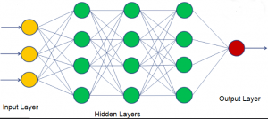
In the case of keras, the model is a neural network consisting of inputs, hidden layers, and a predicted output. Hidden layers are necessary for the model to extract important information about the data and represent the model’s ability to see patterns and connections between features and labels. Each hidden layer consists of a specified number of neurons/nodes, also called hidden units.  Weights are the strength of the connections between neurons of different layers, and can be thought of as a ‘confidence’ level surrounding a certain perceived pattern.

Neural networks find patterns and make generalizations and predictions by being trained on a training data set. Since it is just as important to know how well your model can make accurate predictions on new, previously unseen data, in addition to training sets will be test sets. The test set cannot be included as part of the training set (it has to be new data), but it does has to accurately reflect the trends of the training set.

Another important part of the training process is computing loss. Loss defines how far off the predicted output is from the actual output. During training, the model makes multiple rounds of analyzing the data. Each round is known as an epoch, and this iterative process is what allows the data to learn and develop patterns. Ideally, as the model trains and the number of epochs increases, the total loss should rapidly decrease at first, then flatten out until it converges on a minimum loss. This process of training and minimizing loss is known as gradient descent optimization. The speed at which the model is able to converge on a minimum loss is known as the learning rate. 

There are complications with training neural networks. One important one is the idea of overfitting, which occurs when  the model is more accurate at predicting the training set than on new data its never seen before, and occurs when you train the model too much. Overfitting can be fixed using various methods, which will be discussed later in this post. 

keras with TensorFlow:

The first step before creating any model on tensorFlow is to download the necessary libraries. A common library that is used is pandas, which uses the classes DataFrame and Series to break down numerical data into neat columns and rows.

from __future__ import absolute_import, division,

import matplotlib.pyplot as plt
import pandas as pd

import tensorflow as tf
from tensorflow import keras
from tensorflow.keras import layers

print(tf.__version__)

Next, you must define your training set and data set, separating the features from the labels. The following example is from a categorical model type.

categorical_example = yourdata.categorical_example

(train_data, train_labels), (test_data, test_labels) = yourdata.load_data()

In most cases, some sort of data preprocessing is necessary before training the neural network. For example, if the data is a set of  images of handwritten single digit numbers, with each pixel value in the range of 0-255, we must re-scale this to a range of 0-1. The 0-1 scale will later represent whether the pixel is totally full of writing (1) or completely vacant of writing (0), or somewhere in between. This scaling can be used by the neural networks to find patterns, helping it to identify the image as the correct single digit number.

Once the data is preprocessed, keras builds a model by creating the layers in the neural network. The most common type of model is a stack of layers, the tf.keras.Sequential model.

model = keras.Sequential([
    keras.layers.Dense(16, activation=tf.nn.relu),
    keras.layers.Dense(16, activation=tf.nn.relu),
    keras.layers.Dense(1, activation=tf.nn.sigmoid)
])

In this example neural network model, there are 2 hidden layers and 1 output layer. The Dense stands for densely-connected, or fully-connected, neural layers. The number 16 represents the number of nodes (hidden units) in each layer. Increasing the number of nodes can increase the the capacity for the model to quickly train and find patterns, but can lead to overfitting. The last layer is densely connected with a single output node. Using the sigmoid activation function, this layer outputs a float between 0 and 1, representing a probability, or confidence level of a certain category or prediction. 

Another part of building every model is having a loss function, optimizer, and metrics.  The goal is to minimize the loss function, which measures how accurate the model is during training. The optimizer shows how the model is updated based on the data it sees and its loss function.  Finally, the metrics monitors the training and testing sets. Accuracy is a common tool used in metrics, which measures the fraction of data that have been correctly classified or predicted.

model.compile(optimizer='insert type of optimizer here', 
              loss='insert loss function, often mean_squared_error',
              metrics=[' insert type of metrics, often accuracy'])

Once we have built the neural network, we are ready to train it. A very basic example is shown below, with the number of epochs chosen by the user. Increasing the number of epochs can help the model train but can also lead to overfitting.

model.fit(train_data, train_labels, epochs=5)

We must also evaluate how well the model can make predictions by testing it with the testing data set.

results = model.evaluate(test_data, test_labels)

Creating visuals, such as a graph representing loss by number of epochs, can be a useful tool for analyzing the model and determining if overfitting is an issue.

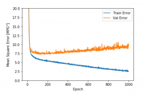
In the graph above, orange is the testing or validation set error and blue is the training error. Notice how error is significantly higher with the test data. This is an example of overfitting.

Fixing Overfitting: 

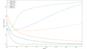
There are multiple ways to fix the common issue of overfitting, in which the model is unable to accurately make predictions about new sets of data. One strategy is to decrease the number of nodes in each hidden layer. While decreasing the number of nodes restricts the computational capacity of the network, it forces the network to only find the most common patterns and make more generalizations, which fits better to new data. The following graph is an example of decreasing and increasing the number of nodes, with blue as the baseline model, green as the bigger model, and orange the smaller model. Notice that the bigger model trains much more rapidly (solid lines), but the smaller model has a much smaller error (dotted lines).

Another way to tackle overfitting is to reduce the number of epochs. Usually, overfitting will occur when there is too much training, allowing the model to find too many patterns specific to the training set. Decreasing the number of rounds of analyzing the data set (epochs) can help fix this problem. The final method is more complex. This method, known as regularization, involves restricting  the quantity and type of information your model can store. Like decreasing the number of nodes, these restrictions force the model to focus only on the most common patterns and to make more generalizations

References:

https://www.tensorflow.org/tutorials/

https://developers.google.com/machine-learning/crash-course/first-steps-with-tensorflow/programming-exercises

https://colab.research.google.com/notebooks/mlcc/intro_to_pandas.ipynb?utm_source=mlcc&utm_campaign=colab-external&utm_medium=referral&utm_content=pandas-colab&hl=en#scrollTo=WrkBjfz5kEQu

https://www.datacamp.com/community/tutorials/neural-network-models-r

Confocal Imaging

Confocal imaging is an alternative to standard optical microscopy, such as conventional widefield microscopy or even Fourier Ptychographic microscopy. It poses an advantage over these forms of microscopy when imaging thick, fluorescent biological samples, such as living cells or tissues. Living cells and tissues are often stained with fluorescent dyes to better view them in a low contrast background, but this poses certain challenges. When imaged by a conventional form of optical microscopy, fluorescence emitted from other parts of the specimen that are not being imaged can interfere with the resolution of cells or tissue that are in focus, causing a phenomenon called “out of focus” glare. This is especially prominent in specimens thicker than 2 micrometers.

Confocal imaging is able to minimize out of focus glare and has an increased resolution for florescent labeled biological samples as opposed to conventional optical microscopy.  Unlike widefield microscopy, which illuminates the entire biological specimen in uniform light, confocal imaging utilizes a laser that emits a focused beam of light to one particular point of the specimen. This light is scanned across the specimen in optical sections, leading to increased resolution without physically separating the specimen into sections, which is an invasive technique that would be required for widefield microscopy for increased resolution. By focusing the source of light on a specific point of the specimen, the illumination intensity drops off sharply for the rest of the specimen that is not in focus, reducing out of focus glare.

The drawback of confocal imaging is it can have poor temporal resolution. This is due to the fact that the light beam is focused to a small point less than a cubic micron is volume, so analyzing the whole specimen would require multiple images as the laser beam analyzes each optical section. In addition, in order to maintain better images for confocal imaging, it is optimal to reduce the power of the microscope when a high numerical aperture is being used, but this limits the speed of acquiring the image.

A possible approach to increasing the temporal resolution of confocal imaging while maintaining a high resolution would potentially be to implement a deep learning algorithm which could speed up the image acquisition time or reduce the number of images required for the given specimen. Attempts with deep learning have been made, such as UCLA’s technique of transforming  confocal images into a super-resolved image that matches the resolution of stimulated emission depletion (STED) microscopy. This super-resolution of confocal imaging uses a deep neural network that successfully increases temporal resolution while maintaining or even increasing the space-bandwidth product.

References:

S. Paddock, T. Fellers, and M. Davidson. “Introductory Confocal Concepts.” MicroscopyU (2019).

“Confocal Imaging.” University of Wisconsin (2019).

H. Wang, Y. Rivenson, Y. Jin, Z. Wei, R. Gao, H. Gunaydin, L. Bentolila, and A. Ozcan. “Deep Learning Achieves Super-Resolution in Fluorescent Microscopy”. University of California, Los Angeles. 1-6. (2018).