3D Fourier Ptychography Optimization

Liquid lenses are a helpful technology to overcome depth of field. Many cameras are often limited by the aperture size and resolution of the lens system, however with continuous focusability over a specified focal range, tunable liquid lenses allow for custom-tuning and optimal performance. Applications of tunable lenses include machine vision inspection systems, unmanned aerial vehicles, and measurement and dimensional rendering.

There are two main types of liquid lenses: focus-tunable lenses and variable focus liquid lenses. Focus-tunable lenses consist of a liquid optical-grade polymer that is mounted in a robust casing and is protected by two windows. These focus-tunable lenses can be either manually-focused by rotating the outer ring and manipulating the focal length, or optical power, which changes the shape from convex to concave, or they can be electrically-focused by applying a control voltage and changing the lens’ radius, which adjusts the focal length within a range of +50mm to +120mm. Variable focus liquid lenses operate via a slightly different process, called electrowetting, which is the use of electric fields to control the wetting properties by applying a voltage to increase the overall curvature, shape, and optical power of the liquid lens. Nevertheless, variable focus liquid lenses are not ideal to work with, since they are small and difficult to integrate with existing objectives., which is why I will focus on the former in this post.

Electrically-focused tunable lenses (Figure 1) provide a single-lens solution for focus and zoom objectives and eliminates the need for a multi-lens system. The lens costs between $300 and $500 and according to Edmund Optics, producer of optics and imaging technology, this device can replace the functionality of a complete lens kit in the laboratory setting. The lenses quickly adjust focus to accommodate objects located at differing working distances and thus are an ideal innovation for imaging applications that require rapid focusing, high throughput, and depth of field. 

As an example, in Stay Focused! Auto Focusing Lenses for Correcting Presbyopia, Elias Wu develops active glasses for attenuating presbyopia, far-sightedness that causes the loss of the eye’s ability to focus actively on nearby objects, by employing auto-focusing lenses (ie. focus-tunable lenses) alongside a calibration-free eye-tracking method (ie. TrackingNet). The setup consists of a ski goggle-like headset with an adjustable lens holder and adjustable eye tracking mount. This device takes in data from the eye tracking cameras and runs it through TrackingNet, a deep convolutional neural network, that implements pretrained models and a multi-layer fully-connected module. This software helps to streamline the auto-focusing lens procedure.

The goal of the paper is threefold: stabilizing the frame and mount so that users could wear it securely, rendering the lens and camera within the frame adjustable, and managing the cables needed to properly operate the headset. In these regards, Wu reports that overall, the headset satisfies these three criteria, however, in regards to the software, it does not yield the best results, which may be attributed to the use of the MSE loss function, when a simple L2 loss may be better. Moreover, the ResNet-50 features convolutional layers that are optimized for classification and thus may not be suited for this type of application in which the gaze position from images of the eyes needs to be found. Most notably, Wu found that the fluid-filled tunable lenses are quite bulky and also have visible distortion around the edges of the lens (Figure 2).

Figure 1: Focus-tunable liquid lenses (Edmund Optics)

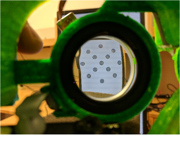
Figure 2: Distortion along edges of auto-focusing lenses (Elias Wu)

Computational imaging-  involves the joint design of imaging system hardware and software to indirectly form images from measurements using algorithms and utilizing a significant amount of computing, overcoming hardware limitations of optics and sensors, such as resolution and noise [1].

Deep learning- a subset of machine learning. Allows machines to solve complex problems even when using a data set that is very diverse, unstructured and inter-connected. Involves two phases: training and evaluation of deep neural network [2].

TensorFlow- an interface for expressing machine learning algorithms, and an implementation for executing such algorithms [3].

Convolutional Neural Network- a class of deep neural networks, most commonly applied to analyzing visual imagery.

Ground Truth- In machine learning, the term “ground truth” refers to the accuracy of the training set’s classification for supervised learning techniques. The term “ground truthing” refers to the process of gathering the proper objective (provable) data for this test. Evaluation campaigns or benchmarking events require a consistent ground truth for accurate and reliable evaluation of the participating systems or methods [4].

Physical pre-processing technique- the function relating low-resolution images to their high-resolution counterparts is learned from a given dataset, which is then used to modify the imaging hardware. By using prior knowledge gained from static images, we avoid redundancy in information collection by physically preprocessing the data [5].

Super-resolution problem- converting low-resolution images to higher resolution.

Space–bandwidth-product (SBP)- a measure of the information a signal contains and also the rendering capacity of a system. Is proportional to the product of the field-of-view and resolution [2]. Includes spatial resolution, field-of-view and temporal resolution.

Spatial resolution– refers to the number of pixels within a digital image. The greater the number of pixels, the higher the spatial resolution.

Field-of-view- the maximum area visible through a camera lens or microscope eyepiece at a particular position and orientation in space.

Temporal resolution- the time to take the multiple measurements of the cross-section and then reconstruct the image.

High-throughput imaging- automated microscopy and image analysis to visualize and quantitatively capture specimens; or real-time live imaging.

Fourier ptychographic microscopy- a computational imaging technique in which variable illumination patterns are used to collect multiple low-resolution images which are then computationally combined to create an image with resolution exceeding that of any single image from the microscope, but has poor temporal resolution [5].

Light field microscopy- a technique that records four-dimensional slices of the five-dimensional plenoptic function by applying an appropriate ray-space parametrization. In many cases, microlens arrays (MLAs) are used in the intermediate image plane of optical instruments to multiplex 2D spatial and 2D directional information on the same image sensor [6].

3D phase microscopy: interferometry-based technique- images are first taken interferometrically to directly record both phase and amplitude information of the scattered field. Next, a tomographic reconstruction algorithm is devised to recover the sample’s 3D refractive index distribution.This typically requires additional specialized and expensive hardware, which is not always compatible to standard microscopes [7].

3D phase microscopy : intensity-only technique- employ tomographic phase reconstruction from intensity-only measurements.  However, changing focus not only requires mechanical scanning, but also increases the acquisition time and data size, both of which are undesirable for high-throughput applications [7].

Optical multiplexing- way of sending multiple signals or streams of information over a communications link at the same time in the form of a single, complex signal. A single LED illumination pattern that allows the information from multiple focal planes to be multiplexed into a single image [8].

References

[1] Waller, L. & Van Duzer, T. (2017). Computational Microscopy. CITRIS.

[2] Cheng, Y., Strachan, M., Weiss, Z., Deb, M., Carone, D., & Ganapati, V. (2018). Illumination Pattern Design with Deep Learning for Single-Shot Fourier Ptychographic Microscopy.

[3] Abadi, M., Agarwal, A., Barham, P., Brevdo, E., Chen, Z., Citro, C., Corrado, G., Davis, A., Dean, J., Devin, M., Ghemawat, S., Goodfellow, I., Harp, A., Irving, G., Isard, M., Jia, Y., Jozefowicz, R., Kaiser, L., Kudlur, M., … Zheng, X. (2016). TensorFlow: Large-Scale Machine Learning on Heterogeneous Distributed Systems.

[4] Foncubierta Rodríguez, A., & Müller, H. (2012, October). Ground truth generation in medical imaging: a crowdsourcing-based iterative approach. In Proceedings of the ACM multimedia 2012 workshop on Crowdsourcing for multimedia, 9-14.

[5] Robey, A., & Ganapati, V. (2018). Optimal Physical Preprocessing for Example-Based Super-Resolution. https://doi.org/10.1364/OE.26.031333

[6] Bimber, O. & Schedl, D. (2019). Light-Field Microscopy: A Review. Journal of Neurology & Neuromedicine, (4)1, 1-6. https://doi.org/10.29245/2572.942X/2019/1.1237. 

[7] Ling, R., Tahir, W., Lin, H., Lee, H., & Tian, L. (2018). High-throughput intensity diffraction tomography with a computational microscope. Biomedical Optics Express, 9(5), 2130–2141. https://doi.org/10.1364/boe.9.002130

[8] Cheng, Y., Sabry, Z., Strachan, M., Cornell, S., Chanenson, J., Collins, E., & Ganapati, V. (2019). Deep Learned Optical Multiplexing for Multi-Focal Plane Microscopy.

Multiplexed Structured Image Capture (MuSIC): Applications for High-speed Imaging and Field of View Extension

Authors: M. Gragston, C. Smith, W. McCord, Z. He, N. Williamson, Z. Zhang.

In this talk, Mark Gragston presents a specific computational imaging technique, similar to structured illumination, in which a unique periodic patterning of light, or spatial frequency modulation, is utilized right before recording in order to encode images into a single exposure. This technique is called Multiplexed structured image capture (MUSIC) and it is essentially exchanging spatial resolution for extra frame storage. Advantages of MUSIC includes its very broad imaging speed range, therefore making it scalable. However, it is limited by the image sequence depths, or the number of frames one can store. Nevertheless, it is useful for field of view extension, where a desired full image is acquired from smaller multiple fields of view, as well as high-speed imaging applications, such as in aerospace photography.

Phase Imaging with Computational Sensitivity (PICS)

Author: G. Popescu

Professor Gabriel Popescu, from the University of Illinois, presents on the value in using phase, rather than intensity, for imaging biological structures as well adding specificity to the phase imaging technique.

Fluorescence microscopy has been used heavily for decades in cell biology, however, the process of staining or labeling cells, which involves the injection of dyes and fluorophores, might exert ill effects on cellular functions. A potential solution is Quantitative Phase Imaging (QPI), which allows for label-free imaging that is nondestructive, fast, and quantitative. QPI has many applications such as diffraction tomography, quantifying cell growth, diagnosing cancer, and much more.

The innovative microscopy technique that Dr. Popescu’s lab has developed is a combination of quantitative phase imaging and Artificial Intelligence and enables information about unlabeled live cells to be gathered with high specificity and this technique is called Phase Imaging with Computational Specificity (PICS). Another method is SLIM (spatial light interference microscopy) as well as GLIM (gradient light interference microscopy), which generate QPI data to which deep learning is applied. One benefit is that both SLIM and GLIM can be added onto existing microscopes and are thus compatible with the fluorescence channels, providing simultaneous phase and fluorescence images from the same field of view. Moreover, this novel approach is a good substitute for a few frequently used tags and stains, thereby removing the difficulties associated with chemical tagging and instead allowing for the non-destructive quantification of the growth of cells over multiple cell cycles.

DiffuserCam: computational microscopy with a lensless imager

Author: L. Waller

Laura Waller addresses the canonical lens imaging problem and suggests taking a camera, removing its lens and replacing it with another scattering element (such as double-sided tape), pointing the sensor at the world, and taking a picture. From this image, Dr. Waller and colleagues can solve an inverse problem to reconstruct the scene.

This idea is a way to replace bulky hardware that is often required for 3D imaging, with a more compact and inexpensive single-shot lensless system. The easy-to-build DiffuserCam consists of a diffuser, or a smooth random optical surface, placed in front of a standard 2D image sensor. Every 3D point within the scene, or volume of interest, creates a unique response on the sensor. In order to solve the large-scale inverse problem, Waller uses a physical approximation and simple calibration scheme. 

However, the issue with this off-the-shelf diffuser is that there are areas that are in between focus spots that are not fully dark, which causes ill-posed SNR deconvolution. So after experimenting with randomly spaced microlenses that focus to multiple spots which are then randomly distributed such that ambiguity is avoided and there is no repeating pattern when the point in the scene shifts.

This is a particularly important development for microscopy, in which live samples are often used and fast imaging is therefore desired along with high resolution across a large volume. Some of the numerous applications that the speaker demonstrates include whole organism bioimaging and neural activity tracking in vivo.

Defining the Digital Camera

Author: D. Brady

Professor David Brady’s research focuses on issues related to the nature of the digital camera and in this talk he goes on to analyze the limitations of digital photography and proposes a new strategy to greatly improve the technology.

For the last 100 years, the main design of the digital camera has not changed significantly: it consists of a camera back and a removable lens. Yet Dr. Brady argues that this model is no longer viable and puts forward an innovative model of his own. Instead of employing a single lens, this new digital camera will be composed of an array of microcameras in which the lens does not form the image, but rather the image is formed computationally. Moreover, the camera must contain a computer in order to run the sophisticated and complex software. The third most important aspect of the camera is that it must become a dynamic sampling engine, where data is recorded all the time that does not simply report data captured in one moment in time, but rather over a period of time during which it is collected. This novel device allows us to explore the world in a much richer way than with traditional media. Some challenges the technology faces include rendering it inexpensive to make it and lowering the processing power per pixel.

An example of this technology being put into action is the Aqueti Mantis Camera, which uses an array of microcameras and carries out most of the video processing. These are actually programmable within the camera head and consist of a cloud style architecture where data is captured in the front end by a thin sheet of optics and an array of 10 single board computers on the back end execute video analysis, image warping, and other functions. Applications include security monitoring for airports, train stations, and roadways as well as for virtual travel and sporting events.

Another advantage is that the diversity of the cameras are not just in field of view, but also focal length by using an array of multifocal lenses where each lens varies in focal length, in addition to diversity in color and exposure. The development of the microcamera arrays are still at the very early stages and the manufacturing processes to develop the complex computer designs at the required scale do not currently exist. And so in order to continue innovating and advancing the digital camera, Dr. Brady suggests to be more imaginative when thinking about what a camera ought to do.

Towards a vectorial treatment of Fourier ptychographic microscopy

Authors: X. Dai, R. Horstmeyer, S. Xu, P. Konda

The Ganapati lab uses single-shot Fourier ptychographic microscopy (FPM) to reconstruct a three dimensional map of a given specimen, or biological structure, from fewer images. Our lab has been able to jointly optimize the LED illumination pattern, which lights the specimen underneath the microscope,  in FPM with a reconstruction algorithm, thus allowing for single-shot 2D imaging of a given sample type while still maintaining a high space-bandwidth product; or a combination of high spatial resolution, wide field-of-view, and high temporal resolution. 

However the sample and pupil function, within the image formation model described above, are all described in scalar. In his talk, Xiang Dai presents a new imaging technique capable of reconstructing the absorption, phase, and polarization-dependent properties of a sample all at once without sacrificing spatial resolution or field of view. Capturing and reconstructing a sample’s polarization-dependent features, such as birefringence and anisotropy, necessitates a different calculus, namely Jones Calculus, to describe the light and optical field in vector form. Dai described the system as an LED light which passes through a polarizer, described by a matrix, which then interacts with the specimen. Via 2D Fourier Transform, the vectorial light field then travels to the pupil plane and subsequently through the imaging lens. Next, a 2D inverse Fourier transform disperses the light to the image plane, passes through another polarizer, and lastly, the intensity measurements of the field are recorded by the digital image sensor.

Self-Supervised Joint Learning of Patterns and Matching for Structured Light Depth Estimation

Authors: E. Fletcher, R. Narayanswamy

In this talk, Evan Fletcher presents a machine learning method for single-shot structured light depth estimation. The way it works is the scene is illuminated with a known, fixed pattern with a camera placed a certain distance away from a projector. This causes the position or direction of objects in the scene to appear different when viewed from the projector and the camera, or parallax, and this shift of the pattern in image space is measured at each pixel using an algorithm. Utilizing this image-space shift measurement, Fletcher is able to calculate the scene depth at each camera pixel. The system is able to train the network at the same time as it optimizes the projected pattern via an in-network differentiable rendering layer, resulting in one structured light pattern and a ML matching algorithm and the results indicate a very accurate depth estimation.

The goal of the paper is to develop a computational microscopy technique to be able to quantitatively characterize thick biological samples. More specifically, the authors aim to obtain 3D cellular information, such as phase and absorption, without having to stain, label, or scan the sample.

Using a standard brightfield microscope, biological cells cannot be imaged, as they appear transparent when left unstained. However, the process of staining or labeling cells, which involves the injection of dyes and fluorophores, might exert ill effects on cellular functions. Therefore, a different imaging method is needed in order to reconstruct the internal 3D structure of cells.

3D phase microscopy techniques fall into two categories: interferometry-based or intensity-only. The most commonly used technique from the former category is optical diffraction tomography (ODT), in which a sample is illuminated using various angles of incidence to directly detect the phase and amplitude information of the scattered field. A reconstruction algorithm is used to retrieve the map of the 3D refractive index (RI) distribution to reveal the important optical properties of transparent samples. Nevertheless, this approach is costly due to the need for interferometry and therefore expensive and specialized equipment, which is why the second category, intensity-only phase tomography, is of more interest.

Intensity diffraction tomography (IDT), as Ling et al. describes, employs tomographic phase reconstruction from intensity-only measurements. Previous IDT methods, however, require mechanical scanning, thus increasing acquisition time and data size, result in lower spatial resolution, or necessitate an iterative reconstruction algorithm, which can be computationally intensive. For high-throughput applications, Ling et al. derive a novel technique that is able to overcome all these limitations by employing a motion-free, scan-free, and label-free IDT model that employs a linear forward reconstruction algorithm, has a slice-based framework, and utilizes angled illumination that enables the direct inversion of 3D phase and absorption from intensity-only measurements for weakly scattering samples.

The setup consists of a standard commercial microscope modified with an LED array source in which images are captured with varying illumination angles. From the 2D slices, sliced along the axial direction, the slice-wise phase and absorption transfer functions (TF) are derived at varying depths for each angle of illumination. Next, the reconstruction algorithm performs 3D synthetic aperture with slice-wise deconvolution to produce two 3D stacks, which represent the phase and absorption.

Above, a graphic from Ling et al.’s paper illustrates the experimental setup, data acquisition, 3D reconstruction, and modeling of 4D TFs.

Ling et al. further validate their technique experimentally with dense biological samples including a stained spirogyra sample and unstained MCF-7 cancer cells. With the imaging of the stained 3D sample, as shown below, the authors used all of 89 brightfield images to perform the IDT reconstruction and successfully demonstrate the attainment of axial sectioning.

With the imaging of unstained dense cell clusters, as shown below, the authors use 153 images to reconstruct 22 phase and absorption slices and establish the flexibility and robustness of their technique in reconstructing both dense and thin samples.

Since the model and the first two experiments only account for single scattering, the authors perform a simulation and an experiment to study the effects of multiple scattering, consisting of stacked phase and absorption resolution targets, which are found to be in agreement with each other and with the theory.

In essence, this new framework is shown by the authors to allow for flexible illumination patterning, fast data acquisition, efficient memory, and low computational complexity. Moreover, this system can also be widely adopted by existing microscopy facilities given its potential for broad application with minimal hardware additions or adjustments. This is of particular interest to our lab, given the method’s capability of biological sample reconstruction and may pave the way for many more biomedical imaging applications.

References:

Ruilong Ling, Waleed Tahir, Hsing-Ying Lin, Hakho Lee, and Lei Tian, “High-throughput intensity diffraction tomography with a computational microscope,” Biomed. Opt. Express 9, 2130-2141 (2018).

Note: This post was intended to be published in early March 2020, but was delayed by the COVID-19 pandemic.

After connecting the Arduino to the LED array — via the RGB Matrix Shield — we tried to run some basic color and shape tests to ensure that everything was running smoothly. Unfortunately, we had an issue where only half of the LED array was illuminated properly.

Thus, I began an extensive debugging process. When the 32×32 LED Matrix was receiving power and no data the entire matrix was illuminated (pictured below).

As a result, I suspected that the issue was data related. With either the ribbon cable or the LED Matrix at fault. As such, I unmounted the array and swapped out the ribbon cable. This didn’t solve the issue.

Thankfully, we had another 32×32 LED Matrix in the lab so I mounted the other LED Matrix with the new ribbon cable. This, too, didn’t solve the issue.

Just to be safe, I again swapped the new ribbon cable for the previous ribbon cable. Again, no change.

Having ruled out both the ribbon cable and the LED Matrix itself as issues, I circled back and did a quick sanity check to make sure there wasn’t a flaw in the code that I was running. This was the same code that was run in the summer of 2018 so I assumed it was good, but it never hurts to check. I ran some example code straight from the documentation. This too failed to solve the problem.

Thinking it may be a power issue, I reseated all the power connections in the entire LED Matrix +Arduino setup and then grabbed the multimeter to check that the correct amount of power is being delivered to the matrix. The multimeter confirmed that there was power delivery to the LED Matrix and to the Arduino. I then checked the power supply to make sure that it was rated to deliver the correct amount of amps and volts (it was). Lastly, I used the multimeter to check if the LED Matrix was actually receiving the 5V and 2A it was supposed to be. Pictured below is part of that process.

Frustratingly, the multimeter proved that the LED matrix was receiving 5V and 2A.

Thinking it may be a soldering issue, I brought in our resident electronics specialist, Ed, to look at our soldering work. He confirmed that it looked fine. He also went over my power work and came to the same conclusions that I did. 

At this point, both he and I were pretty stumped.  I don’t think it’s an Arduino issue because the Arduino boots fine. It could be an internal issue with the shield and, if so, I’d need to wire the ribbon cable to the Arduino via jumper wires to double-check. Ed thinks it might be a power issue, but I am skeptical since everything on the multimeter makes sense. 

I planned to go back into the lab and follow up on my hunch, but then Swarthmore College switched to online learning due to the COVID-19 pandemic and I was/am unable to get into the lab to debug any further.

Note: This post was intended to be published in mid-February 2020, but was delayed by the COVID-19 pandemic.

The RGB Matrix Shield has arrived! Like many products from Adafruit, some assembly is required to get the shield up and running.

Unfortunately, none of the current Ganapati lab members had soldered in over a year. So, after a quick refresher, we set about soldering together the RGB Matrix Shield. The first step was to solder on the reset switch, the screw terminals, and the male ribbon connector.

The silkscreen made it very easy for us to ensure that we didn’t solder on any component backward. For example, the notch on the ribbon connector silk screen lined up with the notch on the ribbon connector part. This may seem trivial, but any design choice to lower the chance of failure is much appreciated.

After soldering on the components, the next thing we did was solder on all the header pins. This proved to be slightly annoying because we wanted to ensure that the header pins were orthogonal to the shield PCB in order to eliminate any problems down the road. This was not as easy as we’d hoped it would be.

After some adjustments to our soldering approach, we managed to get all the header pins oriented in an acceptable fashion and completed the shield assembly. Up next, putting all the pieces together.

Note: This post was intended to be published in early February 2020, but was delayed by the COVID-19 pandemic.

At the end of the 2019 Fall semester, I got the dome array set up and working for a short while. Unfortunately, over the winter months, the teensy Arduino managed to break on this dome as well. As such, we decided to “go back to basics” and reimplement the original 32×32 LED matrix because it didn’t have nearly as many technical hiccups.

In the old setup we wired the Arduino directly to the ribbon cable that was connected to the LED array via jumper wires and a breadboard, but — as you can see below — this wiring is a quite involved process.

With a little bit of poking around, I found out that Adafruit sells an RGB Matrix Shield. In fact, they recommend using this shield to connect from an Arduino to a ribbon cable. With this shield, all you need to do is plug in the ribbon cable. Much simpler and less error-prone than working with ~35 jumper wires.

As such, the lab has decided to buy one to connect our arduino to the LED matrix. It is currently enroute as I write this post!