Potential Super Resolution Algorithms for Fluorescence Microscopy: SIM and PSF

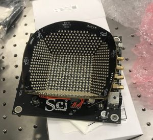
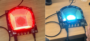
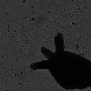
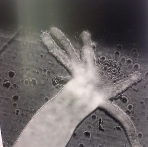
Currently in Ganapati’s lab, we are using Fourier Ptychographic Microscopy (FPM) to image biological samples. This type of microscopy  involves using an LED dome to illuminate the sample in many different illumination angles, allowing for increased image information of the sample with both dark field and bright field images. However, we have come across some challenges with FPM  when using thick or transparent biological samples.

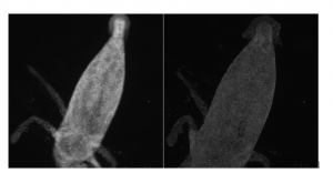
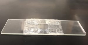
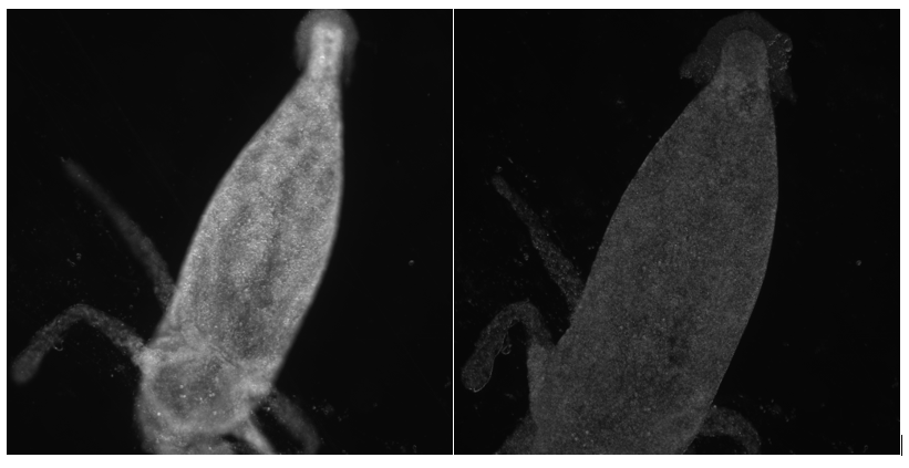
A different type of microscopy that is better suited for thick biological samples is fluorescence microscopy. In florescence microscopy, a sample is stained with various fluorophore dyes, with each dye attaching to different organic or mineral components of the sample. The stained sample is then bathed in intense light, causing the specimen to fluoresce. Because the specimen is now labeled with dyes, it is much easier to visually distinguish different layers of the sample in the image.

There are multiple types of super resolution algorithms that can be used for fourescence microscopy, but two in particular that this lab is interested in are structured light microscopy (SIM) and the point spread function (PSF).

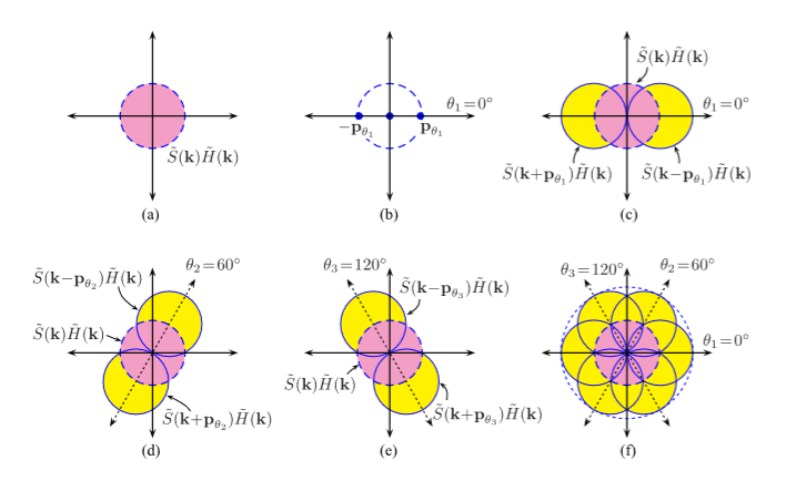
Structured Light Microscopy (SIM):

SIM uses the idea of Moiré‘s Law to aid in super resolution.  Moiré‘s Law can be seen on certain images or on television, producing a wavy pattern. This  Moiré pattern occurs when an object that is being photographed contains some sort of pattern, like stripes or dots, that exceed the resolution of the sensor. This is the same idea as “beats” in sound, and happens as a result of the interference of waves.
SIM technology takes advantage of the Moiré effect in order to extract higher resolution information from the image. In SIM, a striped or dotted illumination pattern is placed just before the sample. This pattern excites the sample, causing it to fluoresce. The interference of the fluorescence emission and excitation waves creates a Moiré pattern, which can be used and interpreted by a computer algorithm to find more spatial information about the image. This in turn allows for the enhancement of the resolution of the image .
A Github repository for a SIM super resolution algorithm can be found here:


Point Spread Function (PSF):

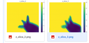
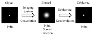
When you are viewing a microscopic fluorescent object under a microscope, the diffraction of light from the emitted fluorescence will cause the object to appear blurred. This blurring, which occurs in both the lateral and depth direction of the object, is known as the point spread function (PSF). PSF tend to have worse blurring in the depth direction, since microscopes tend to have worse resolution in that direction.

In order to minimize the effects of the PSF and reduce blurring, some modifications to the hardware of the microscope can be made, such as having a shorter wavelength of illumination light and  increasing the numerical aperture of the objective lens. On the software side, computer algorithms can “undo” the blurring  caused by the PSF by performing computational deconvolutions, which reverse the effects of the PSF and enhance the resolution of the image.

A Github repository for a PSF super resolution algorithm can be found here: https://github.com/FerreolS/tipi4icy

Resources:

A. Lal, C. Shan, and P. Xi . “Structured Ilumination Image Reconstruction Algorithm.” Department of  Biomedical Engineering,  Peking University. IEEE Journal. 4.(2016).

K. Sring and M. Davidson. “Introduction to Fluorescence Microscopy.” MicroscopyU.

“A Beginners Guide to the Point Spread Function”. Zeiss Microscopy.

A. Lavdas “Structured Illumination Microscopy–An Introduction.” Bitesizebio.com

N. Mansurov. “What is Moiré?” PhotographyLife.com (2012).

LED Dome Patterns Code

We have written a program for the dome that randomly illuminates a fixed number of LEDs at random brightness. Multiplexed illumination is useful in Fourier ptychography because it reduces data collection time without sacrificing information (X). Our code generates several patterns of LEDs and takes one photo for each pattern.

Within the program, we define the number of LEDs to be lit, the number of bright field LEDs, and the number of total LEDs. Currently, we are only illuminating bright field LEDs during imaging. We define the total number of LEDs in anticipation of future imaging that does include the dark field images.

First, we determine the number of patterns to generate by dividing the number of LEDs in use by the number to be lit in each pattern (n). We generate a list of all possible LED indices and shuffle to randomize selection. Then, we assign n indices to each pattern. We pop each index off of the shuffled list, so no index is reused. We use numpy’s randint function to generate a brightness between 0 and 255 for each index.

The inbuilt LED dome commands do not provide for individual LED brightness assignment. Instead, we must reassign the brightness of the entire array before illuminating the desired index. In order to achieve LED patterns that contain many brightnesses, we reset the dome brightness before each LED is illuminated.

We collect and save an image before wiping the current pattern to begin illuminating the next. The section of code used to save the image is not included in the interest of brevity.

for i in range(numPatterns):
   for j in range(len(patterns[i])):

        #Get index of current LED
        light = patterns[i][j]

        #Get brightness of current LED
        intensity = brightness[i][j]

        #Set brightness and illuminate LED
        led_array.command(intensity)
        led_array.command(light)
   
   #Once the full pattern is illuminated, capture a photo  
   time.sleep(0.1)
   mmc.snapImage()

   #Clear the array in anticipation of the next pattern
   led_array.command('x')

Interfacing with the dome occurs extremely quickly. It is reasonable to reset the dome brightness and individually illuminate each LED because, even using this more tedious method, the entire pattern takes only a fraction of a second to display.

The LEDs in our dome are extremely bright, so we are able to significantly reduce the camera exposure time. Previously, we used an exposure of around 2 seconds for illumination by a single LED. For five LEDs of mixed brightness in our new array , an exposure of 0.15 seconds is perfectly sufficient. We have not yet determined the ideal exposure time for an image captured with only one fully bright LED illuminated.

Mounting the LED Dome to the Microscope

Today, we mounted the new LED Dome to our microscope.

Our old array was mounted directly to the microscope stage, which made centering the sample over our objective lens inconvenient. We had to move samples into place by hand because using the stage controls to move samples also caused the LEDs to move and become uncentered.

In mounting our new array, we were careful to uncouple the LED array and the stage. We did this by reattaching the microscope’s condenser arm. This is the vertical piece that supported the microscope’s original illuminator lamp. First, we removed all of the old illuminating elements from the condenser to isolate the vertical condenser arm. Then we used a custom-made L-bracket to mount the optical breadboard plate parallel to the objective lens.

Our plate assembly is pictured below, with a zoomed in view of the L-bracket on the left and a view of the entire microscope, with the plate fixed to the condenser arm, on the right.

We made our L-bracket piece in the machine shop with help from J. Johnson, the machine shop supervisor. He helped us measure the space between screws and determine what diameter of screw was appropriate for each hole. He showed us how to drill holes of appropriate distance and size.

We used metal rods about 1 inch long to suspend the LED dome beneath the plate.

We adjusted the tightness of the screws until the assembly was level. Then we rewired the LED dome and tested some software written yesterday, which divides the brightfield LEDs into a fixed number of random patterns and displays them in turns. This test was successful.


Advantages and Familiarization with the new LED Dome

The Fourier Ptychographic Microscopy (FPM) so far in Ganapati’s lab has been performed with a flat 32×32 LED array.  With a flat array, you can light up one LED at a time to acquire different illumination angles for imaging. However, there are many disadvantages to the current flat LED array set-up. For example, one major issue  regarding the flat LED array is that it is programmed by Arduino, which does not contain memory. When we tried to reprogram the array to light up random multiplexed patterns of LEDs rather than one LED at a time (a change that could greatly reduce data acquisition time), we were unable to do so because the Arduino could not store information on the location of the LED coordinates. In addition, the flat LED is not very bright and contains smaller illumination angles, producing low resolution images that contain less intensity information and therefore decreases the space-bandwidth product (SBP) of the FPM reconstructed images.

By replacing the flat LED array with an LED dome purchased from Spectral Coded Illumination (Sci), many improvements could be made to our current FPM procedure.  We can easily program the dome to produce random multiplexed patterns of LEDs because the LED can be programmed directly through Python, a much more robust and easy-to-use software than Arduino that can easily store information. In addition, each LED is assigned a specific number rather than a x-y coordinate position, making it easier to write programs that access certain LEDs.

Because of the sloped sides of the array, which produces a dome shape, the LED dome can produce much higher angles for dark field illumination, allowing for increased intensity information of images and thus increasing the SBP of the reconstructed high resolution image. In addition, the LED dome is much brighter than the flat LED array, also contributing to higher quality images and better data for reconstruction. Finally, the dome is programmed to sweep through and illuminate LEDs  at a much faster rate than the flat array, significantly reducing data acquisition time.

Once we received the LED dome, we proceeded to download the necessary programs and become familiarized with the various commands for the dome. For instance, the command ‘bf’ illuminates only the brightfield LEDs, which are the LEDs located at low illumination angles and located directly above in sample in the flat roof of the dome. Other examples of commands are shown but not limited to the list below:

‘df’    illuminates only the dark field LEDs.

‘ff’     illuminates all LEDs in the array

‘sb.[r].[g].[b]’   sets the brightness of the array

‘scf’       lights up each LED in the array individually. Takes less than 1 minute to fully scan.

‘x’ clears the array

In the next few days we plan to learn more about setting up the hardware trigger modes for direct communication between the PCO camera and dome. We also plan to design and create a way to mount the LED dome onto the microscope so that we can allow for an automated stage. Currently with our flat LED array, we have the array attached to the stage, confining the lab group to manually moving the slides with our hands rather than having a more precise automated stage system.


Notes from “Image Super-Resolution Using Very Deep Residual Channel Attention Networks” by Zhang et al.

Convolutional neural networks excel at visualization tasks, and are popular for tasks like single image super resolution (SR), where a high-resolution image is generated from a single low resolution input. SR is an ill-posed problem because for any one low resolution image, many high resolution interpretations are possible.

CNNs can learn the relationship between low-resolution images and their high-resolution counterparts. Generally, deeper neural networks are better able to generate these mappings. However, it is important that deep neural networks handle input data efficiently. Otherwise, they waste computational resources on information that will not cause the high-resolution output image to be more detailed or accurate.

Many CNNs developed for SR treat low and high frequency information from input images as equally necessary to computation. Low frequency information, which expresses gradual change in pixel intensity across the image, is easily extracted from low-resolution images. It can be forwarded more or less directly to the high-resolution output. High frequency information is an abrupt change in pixel intensity. It occurs in places of sharp intensity change, like edges. This is the detail that SR attempts to recover in order to generate a high-resolution output.

The network described in this paper, called RCAN (residual channel attention network),  adaptively learns the most useful features of input images. It uses a residual in residual structure to make the extremely deep network easier to train. Long and short skip connections allow the network to forward low frequency information directly toward the end of the architecture. The main portion of the network can therefore be dedicated to learning more useful high frequency information.

Above, a graphic from Zhang et al.’s paper illustrates the architecture of their network.

The RCAN network uses a post-upscaling strategy. Unlike other techniques, RCAN does not interpolate the low resolution input to the size of the output image before feeding it into the neural network. Preemptively enlarging the image increases the computational work that must be done and loses detail. Upscaling as a near-final step increases the efficiency of the network and preserves detail, resulting in more accurate outputs.

The residual in residual (RIR) structure used by RCAN pairs stacked residual blocks with a long skip connection. This allows the authors to have a very deep network (1,000+ layers) without making it impossible to train. They use a channel attention mechanism to emphasize network attention to the most useful information contained within the low resolution input. This most useful information is high frequency detail information, and is isolated by exploiting interdependencies between the network’s feature channels.

RCAN is shown by the authors to outperform other SR techniques, as shown below.

Arduino Illumination Code

We are writing code that switches quickly between LED illumination patterns for rapid illumination.

Our usual illumination strategy saves individual LED coordinates and brightnesses in a .txt file. This text file is parsed by python code and passed into the serial port of the Arduino controlling our LED array. This method is slow because instead of illuminating the entire pattern at one time, LEDs are illuminated one by one.

When we are sequentially illuminating LEDs during data collection, our current strategy works well. We only need a single LED illuminated at any time, and we cannot image too quickly. Our images have a 2s exposure time because our LEDs are not very bright and they have a slow refresh rate. If we image too quickly, we experience banding.

Now, we want to be able to very quickly collect images under multiple specific illumination patterns. It is not efficient to individually illuminate LEDs when many are lit at the same time. Instead, we have written an Arduino program that assigns LED illumination patterns to a full array before illuminating. It takes milliseconds to switch back and forth between two full illumination patterns.

The desired LED illumination pattern is laid out in the style of the 8×8 example below, with individual array values representing the brightness of the corresponding LED.

 int image1[][8] ={
              {0,50,0,50,0,50,0,50},
              {0,70,0,70,0,70,0,70},
              {0,90,0,90,0,90,0,90},
              {0,110,0,110,0,110,0,110},
              {0,130,0,130,0,130,0,130},
              {0,150,0,150,0,150,0,150},
              {0,170,0,170,0,170,0,170},
              {0,190,0,190,0,190,0,190}
              };

This 8×8 array uses a brightness range from 0 to 255. Our full sized 32×32 array has a brightness range from 0 to 7.

We can create multiple illumination patterns and pass them to a function that illuminates the LED array accordingly. First, however, we must determine how best to translate the generated optical element into an Arduino array.

The neural network that generates the optimized optical element saves an npy file of illumination intensities, which are ordered in the same sequence as the LEDs are illuminated during data collection. We could open this npy file in python and examine it, then fill in the corresponding Arduino array by hand. We would prefer a quicker and less tedious solution; for example, we are looking to convert the provided npy file to a type more easily read by Arduino.

Changes in Hydra Imaging Procedure

As we image and pre-process the hydra data, we have continued to encounter unexpected problems, leading us to make changes to our imaging procedure in order to best optimize the output of our data.

The first issue we encountered was the fact that the hydra were being flattened by the pressure of the cover slip while imaging was taking place. This caused the slow degradation of the hydra, causing major differences between image 0 and image 68 (see image below).

Differences between each of the 69 images in each stack, other than the change of position of the light source due to the each illuminated LED, are problematic and result in poor training data for the neural network.  The lab group solved this problem by stacking up double-sided tape on the slides with the cover slip sitting on top, allowing for a 3-dimensional gap for the hydra to rest in during imaging.

While the hydra itself are now better preserved during imaging, we have since come across additional imaging problems.  We tried running our shift-add algorithm,  which takes the low resolution stack of images and analyzes the image at different z-distances (depths), producing different three-dimensional “slices” of the image. However, we found that the resulting image slices were completely saturated with light, producing the yellow image below.

The lab group quickly realized that stray light from the lab room was saturating the images in too much light. In order to eliminate stray light, it is necessary to image either in a dark room or with a cover completely over the FP microscope. The lab group chose to use a large cardboard box as a cover for the microscope and camera. We took more data, ran the shift-add algorithm, and were successfully able to produce image slices of the hydra. Below is a look at an example of an original low resolution image of a hydra and a couple of its resulting slices from the shift-add algorithm.

The final problem, and so far one of the most difficult to solve, is the subtle movements of the water surrounding the hydra in the slide. These small movements of the water, caused by factors such as tiny shaking of the building, so small that they are nearly undetectable, cause the hydra to move ever so slightly in the flowing water. This results in a visual and problematic shift between image 0 and image 68 in a stack (example shown below), producing poor training data for the neural network.

The ideal way to solve this problem is to use a specially designed optical table, which corrects for minute movements and shakes such as these. However, the lab currently is not equipped with an optical table, so alternative attempts at a solution have been made. Currently the lab group is using a tray with small dishes for imaging. We figure that with smaller dishes, the water has no place to move and expand, whereas with the taped slide method, there were empty pockets of space for the water to flow into. The potential drawback with this method is the tray is made of thicker plastic compared to the glass slide, which could possibly produce less clear images.

Hydra Data Pre-Processing Issue

After fixing the issue of keeping the hydras from being flattened by the cover slip, we began collecting low-resolution images of the hydras to start running algorithms for reconstructing a high-resolution image.

We chose a sample data set with one stack of images and ran the Generatescript.py code. By executing the sh file that it created, we ran into a problem in which no high resolution image was generated. To see if the problem lay with the program or the images, we tried running the code with a flatworm data set imaged last summer. This succeeded in producing the high resolution image, confirming that the issue relates to our hydra data somehow.

Currently we suspect that the one stack of data is not sufficient for the pre-processing procedure, so we are currently trying with a five-stack hydra data set for the GenerateScript.py. Once the program stops running, we will see if this is in fact the source of the problem or not.

Hydra Imaging Preparation

Our most recent project involves imaging small, multi cellular aquatic organisms called hydra. This organism is most notably known for its lack of aging since it is comprised mostly of regenerative stem cells. Our hydra are provided by a lab in Swarthmore’s biology department. We were given vials containing about 10 fixed regular and ‘inverted’ hydra. The inverted hydra have been sliced open and turned inside out, providing another perspective of the hydra for imaging. We were also given a pipette, a small glass dish with a hollow in the center, and a stack of cover slips to rest over the hydra.

As we began our imaging procedure, we quickly ran into problems. For instance, because we are imaging with an inverted microscope, there is a hole in the microscope stage over the objective lens. The dish we were given for imaging the hydra  was smaller than the hole in the stage, causing the dish to fall through and have no where to sit.  To fix this,  we acquired a larger dish, which did not have a center hollow.

We prepared hydra samples by pipetting one hydra onto the large dish and resting a cover slip on top. At first, this process appeared to work well. As imaging went on, however, we noticed that the body of the hydra seemed to expand and degrade. Below, we include the 1st and 137th images from one of our imaging datasets.

The hydra appears to have a different shape and density at the end of imaging than it did in the first image.

We brought our imaging results to our contact in the biology lab. We demonstrated our pipetting technique to show that the hydra were not being damaged during slide preparation. We mentioned that we had replaced the small dish with a larger one that had no center hollow because the small dish did not fit on the microscope stage.

The biologist explained that the dish hollow was an important feature that gave the hydra, a three-dimensional organism, space beneath the coverslip. When we applied the coverslip directly on top of our hydra, we were crushing it under the pressure of the cover slip. This caused the degradation we saw in our datasets.

He recommended building our own three-dimensional well for the hydra on a glass slide. By applying several layers of double sided tape on either side of the water droplet containing the hydra, we can raise the coverslip high enough that it does not crush the animal. This should prevent future sample degradation.

Data Collection of Hydras

Now that all the computers are set up except for the one with the monitor that will be using for data processing, we started collecting  low resolution image stacks from the hydras we received from Swarthmore’s biology department.

By placing the hydra into a dish and stabilizing it with a square plastic cover, we are able to observe the hydra under the Fourier Ptychographic microscope and collect photos using the camera.

We took photos with three different diameters of the LED matrix, specifically 9, 11 and 13. By lighting up different ranges of LED lights, we were able to create three low resolution data sets with 1 low resolution stack per diameter. After taking these datasets, we will decided that the 10x magnification is best if we want to be able to image the entire hydra rather than a part of that hydra.

Shift-add algorithms and the iterative reconstruction algorithm will be implemented once the computer with the algorithms is set up.